Embeddings and the Maps We Draw of Them
Second in the series “Understanding LLMs to use them better in management and finance.” It follows QKV Attention (how a Transformer moves information between tokens) and sets up The Final Step (how the final layer reads an answer out of the vocabulary — a relentless search for the best next word). This note is about the thing both the attention machinery and that final read-out quietly depend on: the vocabulary embeddings — what they are, where they come from, and how to look at a space with hundreds of dimensions without fooling yourself. It is written for a reader who is not a computer scientist; the technical terms (token, residual stream, PCA, softmax, …) are collected in the Glossary at the end, and each is also explained where it is first used.
1. What an embedding is — and the chicken-and-egg of finding it
Everyone who has met a language model has met the idea of an embedding: each word (more precisely, each token) is a point in a high-dimensional space, and “nearby” points are supposed to mean “similar” things. The picture is so common that it is easy to skip the question that actually matters for using these models well: where do those vectors come from?
There is a tempting wrong answer, and it is worth naming because it is the mental model most people import from vector databases. In a vector database — the engine behind semantic search and retrieval-augmented generation — you take an already-trained encoder, push each document through it, and store the vector it produces. The encoder is fixed; the vectors are read off it; “similarity” is a property of a model someone else trained earlier. The embedding is an input to your system.
Inside a language model, embeddings work the other way around. They are not downloaded from a standard generator and they are not fixed in advance. They are parameters — the rows of the embedding matrix E — and they are learned jointly with the rest of the model, by the same gradient descent that trains the attention and MLP weights. There is a chicken-and-egg quality to this that is the whole point:
The embedding of a word is whatever vector makes this particular model predict well. The model shapes the embeddings; the embeddings shape the model; they are solved for together.
So when GPT-2 places “king” at some location in its 768-dimensional space, that location is not a statement about the timeless meaning of king. It is a statement about what direction is useful for GPT-2’s next-token predictions, given everything else GPT-2’s weights are simultaneously doing. Train a different model on different data and you get different embeddings, even for the same word.
A fair objection: aren’t the vectors in a vector database also learned? They are — and being precise about this softens the contrast in the right way, because the real difference is not “learned versus not learned.” The encoder behind a vector database is itself a trained neural network — OpenAI’s text-embedding-3, the open sentence-transformers family, or token-level late-interaction retrievers like ColBERT are all optimised models. What differs is the objective they were optimised for. A retrieval encoder is trained so that the similarity between two pieces of text tracks their relevance — exactly the quantity a search index needs. A language model’s embeddings are trained so that the model predicts the next token. Same mechanism (vectors solved for by gradient descent), different goal — and a different geometry results. So the lesson of this section is not “LM embeddings are special because they are learned,” but the sharper: every embedding is shaped by the task it was trained for; there is no neutral, universal embedding you simply look up. The vector you get for king depends on whether you asked “what retrieves documents about kings?” or “what predicts the word after king?”
This is the first thing to internalise, because it explains everything that follows — including why the most natural-seeming way to build embeddings by hand, dictating the axes yourself, does not work.
| Vector-database embedding | Language-model embedding | |
|---|---|---|
| Where it comes from | a pre-trained encoder you call | a parameter learned during training |
| Fixed or learned? | learned by the encoder, then frozen at lookup | learned jointly with all other weights |
| What “similar” means | a property of the encoder’s training | whatever helps this model predict next tokens |
| Role in the system | an input (you store it) | an output of training (the model owns it) |
| Can you choose the axes? | no (encoder decides) | no — and §2 shows that trying breaks the model |
2. The pivot: a cautionary tale about wiring the meaning by hand
Because embeddings are “just” vectors with interpretable neighbourhoods, a very reasonable engineer’s instinct is: why not build them myself? If I know that words differ along a few common-sense axes — gender, age, power, size, whether they are animate, to name a few — why not assign each word a short vector on those axes, feed a small model some sentences, and let it learn the rest? The axes would be human-readable, the space would be tidy, and interpretability would come for free.
This note’s running example was built precisely to test that instinct, and the result is the most useful thing in it. I designed a tiny vocabulary (~40 content words: king, queen, lion, lioness, stag, mountain, pebble, ship…) and a six-dimensional hand-wired latent space — gender, age, power, size, animacy, mobility — with each word assigned coordinates in \{-1, 0, +1\} (king = male/adult/strong/—/animate/mobile; pebble = —/—/—/small/inanimate/still; and so on). From that latent table I generated a corpus of simple definition and comparison sentences (“the king is older than the …”, “a lion is bigger than a …”), and trained a small Transformer (2 layers, 2 heads, d_{\text{model}}=32) on it. The model was never shown the latent table — the experiment was whether, trained on data whose every regularity is a function of those six axes, the model would recover them in its own learned embedding.
It did not. Here is the picture that tells the story.
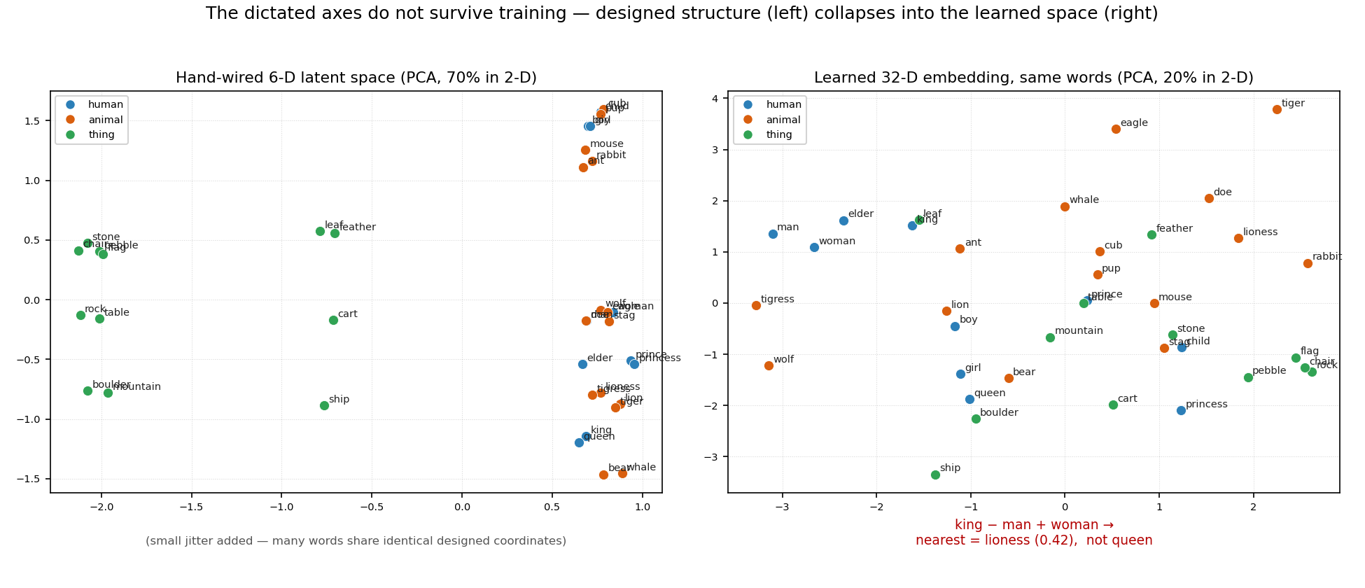
On the left is the hand-wired latent space (the six designed dimensions, projected to 2-D by PCA). It is exactly what you would hope for: clean, structured, the three classes (human / animal / thing) separated, the discrete lattice of designed coordinates visible — its top two principal components capture 70% of the variance, because we put the structure there. On the right is the model’s learned 32-dimensional embedding for the same words, projected the same way. The tidy structure is gone: the classes interleave, the top two PCs capture only 20% of the variance, and — the giveaway — the famous word2vec analogy fails. Computing king − man + woman and asking for the nearest word returns lioness (cosine 0.42), with child and cub next; queen is not in the top five. The model has not learned a clean “gender axis”; it has learned a diffuse blob of feminine-animate mass and a separate male-animate blob, and the arithmetic lands wherever those blobs happen to sit.
By every acceptance test we set in advance, the experiment failed: principal components flat (50% cumulative over six PCs, against a 75% target), zero of six linear probes able to read a latent axis back out at R^2 > 0.8, and only two of five designed analogies recovered. So why does hand-wiring the meaning fail so thoroughly?
2a. The child and the draughtsman
A child asked to draw a person assembles a kit of symbols: a circle for the head, two dots for eyes, a triangle for the nose, a line for the mouth, sticks for the limbs. Each part is a discrete token, drawn on its own, sitting in its own patch of paper, meaning one thing. The picture is a sum of labelled pieces.
A trained draughtsman does the opposite. A single line traces the underside of the eye and, without lifting, becomes the bridge of the nose; one shadow gives the cheekbone and the eye socket at once; whole regions are set not by the outline of a “part” but by tone. No stroke belongs to one feature, and no feature lives in one stroke. The face emerges from the configuration of marks as a whole — which is the central lesson of Betty Edwards’ Drawing on the Right Side of the Brain: the beginner’s real obstacle is cognitive, not manual. The mind insists on what it already knows — “an eye is an almond with a circle in it” — and stamps that symbol onto the page, drowning out what the eye reports. To draw, you switch off the symbol-maker and let the subject come out of the whole.
This is exactly the difference between the two ways of holding meaning in a vector. When I fabricated embeddings by hand — one axis for gender, one for age, one for power, one for size — I was drawing like the child: one feature per symbol, each concept walled off on its own dedicated dimension, the vocabulary a kit of labelled parts. It trained poorly, and the failure was not a bug to fix; it was the model refusing to draw like a child. A set of embeddings that works is drawn like the artist: each direction in the space serves several meanings at once, and each meaning is spread across many directions. Concepts are not parked on private axes — they are shared out over the available strokes, and the word comes out of the whole.
Hand-wired embeddings draw a face the way a child does: a symbol per part. Learned embeddings draw it the way an artist does: every line doing several jobs at once, no part living in a single stroke.
2b. From symbols to distribution and superposition
The analogy is worth pinning exactly where it holds. It explains why a working code is distributed rather than symbolic — meaning smeared across the strokes instead of filed under labels. It does not, on its own, explain the stronger and more specific fact that a model stores more features than it has dimensions, tolerating a little interference to do so. That step is not about artistry but about geometry: it is possible only because a high-dimensional space has room for very many almost-non-overlapping directions. The drawing is the intuition; superposition is the mechanism — which is where we turn next.
Back to our question: why does hand-wiring the meaning fail? There are four linked reasons, and together they are the core lesson of this whole note.
Hand-wiring forces axis-aligned concepts — one meaning per dimension. My design said “dimension 1 is gender, dimension 3 is power.” But a learned embedding has no reason to put one concept on one coordinate axis. Which brings us to:
Real features are distributed, and packed in superposition. Gradient descent does not store “gender” on axis 1. It stores many features as directions — often many more directions than there are dimensions — squeezed in at angles chosen so they interfere with each other as little as possible. A direction that means “feminine” can be a diagonal combination of dozens of coordinates, sharing space with hundreds of other such diagonals. This packing of more features than dimensions is called superposition, and it is the normal state of affairs in a self-organising model trained to minimise empirical error, not a pathology.
Descent wants freedom, not your axes. The reason it packs things this way is that it is optimising for prediction, and the geometry that predicts best is the one that places each useful direction where interference is lowest — not the one a human finds legible. Dictating the axes removes exactly the freedom the optimiser needs. A handful of clean symbolic dimensions simply cannot supply the statistical degrees of freedom a model uses to fit language.
It is the same phenomenon as distributed coding. Neuroscientists have long argued that a concept in the brain is carried by a population of neurons rather than a single “grandmother cell”; interpretability researchers find the same in networks — individual units are usually not cleanly interpretable. The reason you cannot read meaning off a single dimension of a real embedding is the same reason hand-wiring one meaning per dimension fails: meaning does not live on the coordinate axes. It lives in directions, and the axes are an arbitrary basis.
The lesson, stated plainly: if you want embeddings that work, you have to give up wiring the meaning by hand. The price of a model that predicts well is a space whose coordinates are not individually meaningful. (This particular toy also illustrates a narrower trap — a corpus mechanically generated from a feature spec gives the model nothing to do but memorise the templates, so it never has to infer the latent axes at all. But the deeper point stands for real models trained on real text: their useful structure is distributed, not axis-aligned.)
Is this too strong? It is worth checking against the literature before generalising, because the assertion is forceful — and three well-known results sharpen it rather than overturn it. First, sparse autoencoders trained on a model’s activations (Anthropic’s Towards Monosemanticity, 2023; Cunningham et al., 2023) do succeed in recovering clean, human-readable features — but they recover them as directions teased out of the superposition, which is precisely the claim that the meaning is present yet not aligned with the raw axes. Second, injecting hand-built structure is not worthless: retrofitting word vectors toward a lexicon or ontology (Faruqui et al., 2015) measurably improves them — but it adjusts already-learned vectors, it does not replace learning with a dictated table, which is the thing that fails. Third, the difficulty is principled: recovering clean, axis-aligned factors without strong inductive biases is provably impossible in the unsupervised case (Locatello et al., 2019). So the careful statement is not “structure never helps” — it sometimes does — but: you cannot hand-author the whole embedding and freeze out the model’s freedom to place features where prediction wants them, and what a model learns will be distributed rather than one-concept-per-axis. That is the robust core, and it is what the toy demonstrates.
3. What real embeddings are actually like
So the dimensions are not individually meaningful, and there are a lot of them: their number d_{\text{model}} is 768 in GPT-2 small, 4096 in a typical 7-billion-parameter model, 12,288 in GPT-3 (175 billion parameters, one of the most-studied LLMs), and larger still in frontier models. Two consequences follow immediately, and they set up the rest of the note.
Reading single dimensions is hopeless — partly because there are hundreds or thousands of them (trans-human to eyeball), and more importantly because, per §2, an individual coordinate usually means nothing. The interesting structure is in combinations of dimensions — in directions.
Therefore we need compressed views. To see a high-dimensional space we must squash it down to two or three dimensions we can plot. And here is the part that is easy to forget: every way of squashing is a choice of what to preserve, and therefore a choice of which question you are asking. A 2-D map is never “the” embedding space; it is an answer to one question about it. Pick the wrong method for your question and the map will mislead you with total confidence.
The next section lays out the three families of method you will meet, what question each one answers, and — just as important — what each one quietly destroys.
4. Three ways to look at an embedding space
The three workhorses are concept directions (you bring the meaning), PCA (the data brings the directions of greatest spread), and t-SNE/UMAP (the data brings local neighbourhoods, nonlinearly). They differ on every axis that matters:
| Concept directions / Gram-Schmidt | PCA | t-SNE / UMAP | |
|---|---|---|---|
| Supervised? | Yes — you choose the axes | No | No |
| Linear? | Yes | Yes | No |
| A true projection? | Yes (onto chosen axes) | Yes (onto top eigenvectors) | No — a learned 2-D embedding |
| Readable directions / arithmetic? | Yes — that is the point | Sort of (PC axes have a sign) | No — axes mean nothing |
| What it preserves | your chosen contrasts | global variance | local neighbourhoods only |
| What it destroys | everything off your plane | small-variance structure | global geometry, distances, density |
| Best question | “where do words fall on this meaning?” | “what are the biggest directions of spread?” | “what clusters together locally?” |
To make the comparison concrete, here is one embedding space — the 28-token vocabulary of our trained dialogue-game model (a tiny word-level Transformer, 2 layers × 4 heads, d_{\text{model}}=64, that plays a turn-taking “calling game”: Pietro chiama Paolo, with epithets that depend on who calls whom) — shown all three ways at once. The vocabulary splits into roles: players (Pietro, Paolo, the numbers 1–8), epithets (Tarso, Cefa, capo, vice), verbs (chiama, perde), absurd distractor words, and special tokens.
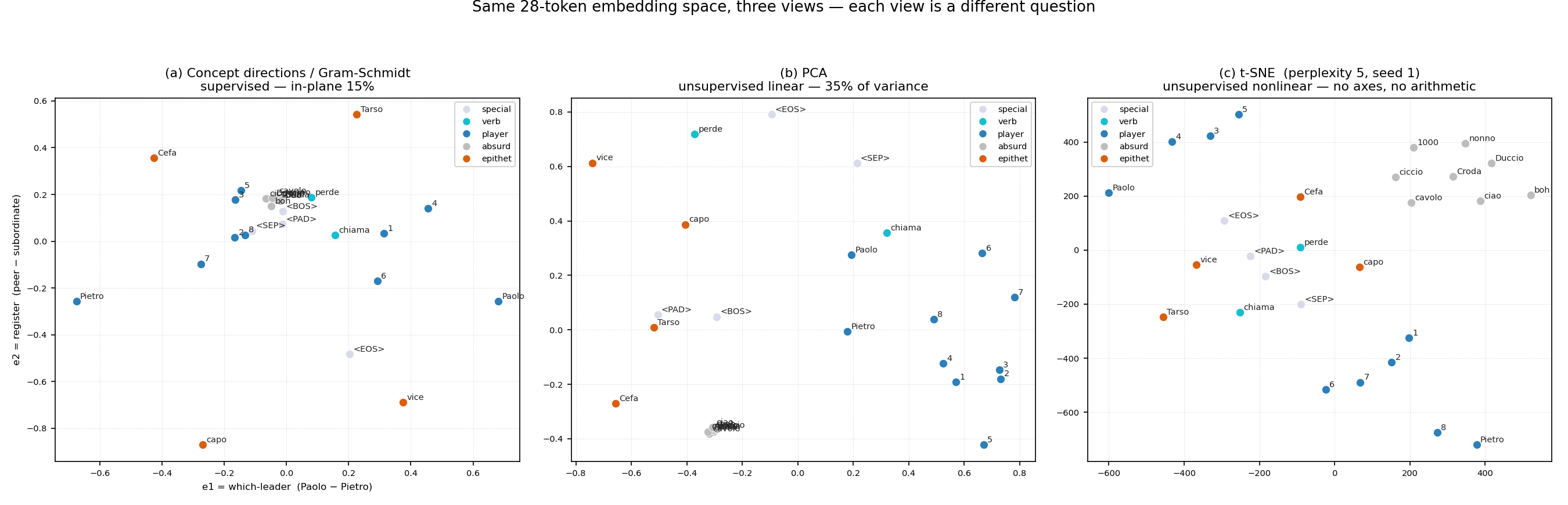
Same 28 points, three pictures, three different stories. Now each method in turn.
4a. Concept directions — you bring the meaning
The most honest method is also the most opinionated: you decide what the axes mean. You pick a direction in embedding space that stands for a concept — either by naming a token (“the direction of Tarso”) or, more usefully, by taking a difference of tokens (“Paolo minus Pietro” = the which-leader direction), then orthogonalise a second concept against the first (Gram-Schmidt) so the two axes are independent, and read off where every word lands. The leftmost panel (a) of the figure above uses $e_1 = $ (Paolo − Pietro) and $e_2 = $ (peer epithets − subordinate epithets): the epithets fly to the corners exactly as their roles predict.
This is the king − man + woman ≈ queen world, and it is the method this project already uses elsewhere — applied not to the vocabulary but to the residual stream, the running vector the model updates token by token (see the QKV note). Because our model ties its embedding and unembedding matrices (The Final Step develops why this makes the dictionary the model searches literally the embedding matrix), moving the residual toward a token’s embedding direction is raising that token’s probability. So we can build a Gram-Schmidt plane from two embedding rows and watch the prediction travel across it. The next figure is a separate, single-panel plot — not one of the three panels above, and built on a different pair of axes:
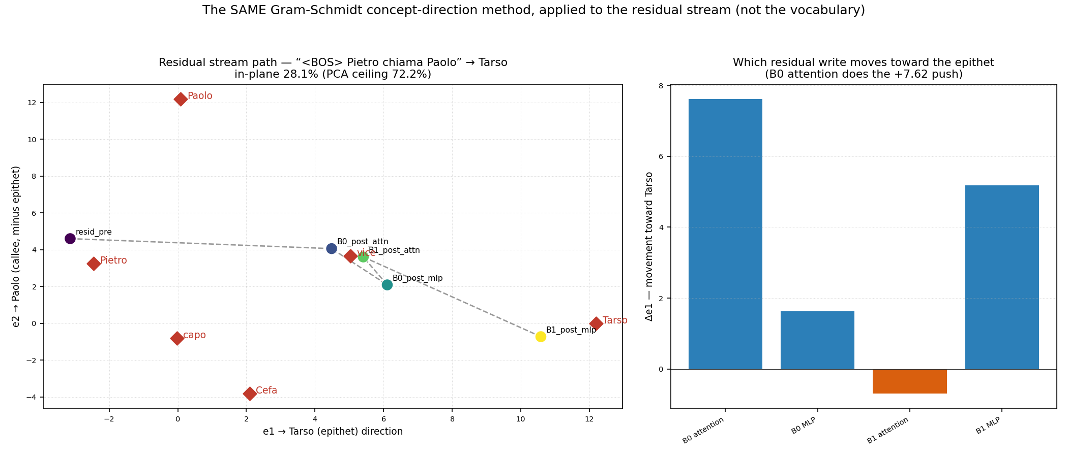
For the prompt <BOS> Pietro chiama Paolo, the model must emit Paolo’s epithet, Tarso. Note this is a different concept plane from panel (a): here e_1 is the Tarso direction itself and e_2 is the callee Paolo with its Tarso-component removed (Gram-Schmidt again, on a different pair of rows) — chosen because we are now tracking the prediction of Tarso, not laying out the whole vocabulary by leader and register. The residual starts near the called name and migrates across the plane toward the Tarso direction as the layers run (the e_1 coordinate climbs from −3.1 to +10.6), and decomposing the path by which write moved it shows that the attention block in layer 0 does the +7.62 push toward the epithet — pinning the behaviour to a specific component, the same kind of causal claim the QKV note’s ablation appendix makes. The point for this note: concept directions are supervised. They show you exactly what you ask about and nothing else.
That last clause is the catch, and the numbers make it honest. The concept plane in panel (a) captures only 15% of the vocabulary’s spread, and the residual plane captures 28% of the trajectory’s spread (against a best-possible 72% — see §4b). A supervised plane is chosen for meaning, not for variance, so it generally is not where the data spreads most. That is a feature, not a bug — but it means you are seeing your hypothesis, not the data’s own structure. Caveat: the famous analogies are partly fragile and cherry-picked (the literature has known this for a decade — see §7); they are cleanest on classic static word embeddings and patchier inside trained language models, as our own king − man + woman → lioness already warned.
4b. PCA — the data’s own biggest directions
PCA asks a different, unsupervised question: along which directions does the data spread most? It finds them by an eigen-decomposition of the centred data (a single svd call), and projects onto the top two. Unlike concept directions, you bring no hypothesis; unlike t-SNE, it is a genuine linear projection — the axes have a fixed meaning, you can read coordinates off them, and (with care) do arithmetic.
Panel (b) above is the PCA of our 28 embeddings; its top two components hold 34.7% of the variance, top four 55.3%. That single number — “only a third of the structure fits in the best possible 2-D linear view” — is itself the most useful thing PCA tells you, and it is honest in a way a t-SNE plot never is: it quantifies how much you are not seeing.
But PCA has a caveat that bites constantly and is widely under-appreciated: variance is not meaning. The directions of greatest spread are very often boring — token frequency, vector norm, or positional artefacts — rather than clean semantics. In word embeddings this is so reliable that a standard preprocessing trick (“All-but-the-Top”, §7) is to delete the top few PCs because they encode frequency. The practical defence, which our tooling also offers, is to project the rows onto the unit sphere first (a “cosine” view): that removes the magnitude/frequency effect and lifts our 2-D fraction from 34.7% to 43.5%, placing rare tokens by their direction instead of letting their small norm collapse them to the centre.
4c. t-SNE (and UMAP) — local neighbourhoods, with loud caveats
t-SNE answers a third question: which points are each other’s nearest neighbours? It is nonlinear and local — it tries to keep neighbours together while caring nothing about anything else — and it usually produces the prettiest, most cluster-y pictures, which is exactly why it is the most dangerous. Four caveats deserve to be stated loudly, because every one of them is routinely violated in practice:
It is not a projection. There are no axes, so a t-SNE plot has no readable directions and supports no arithmetic. “Right” and “up” mean nothing. (UMAP, the popular faster cousin, shares this — and additionally is not designed to preserve global structure either, despite a common belief otherwise.)
Inter-cluster distances are meaningless. Two clusters drawn far apart are not “more different” than two drawn close. The gaps between blobs carry no information.
It is stochastic. A different random seed gives a different layout. Here is the same 28-token data, same perplexity, two seeds:
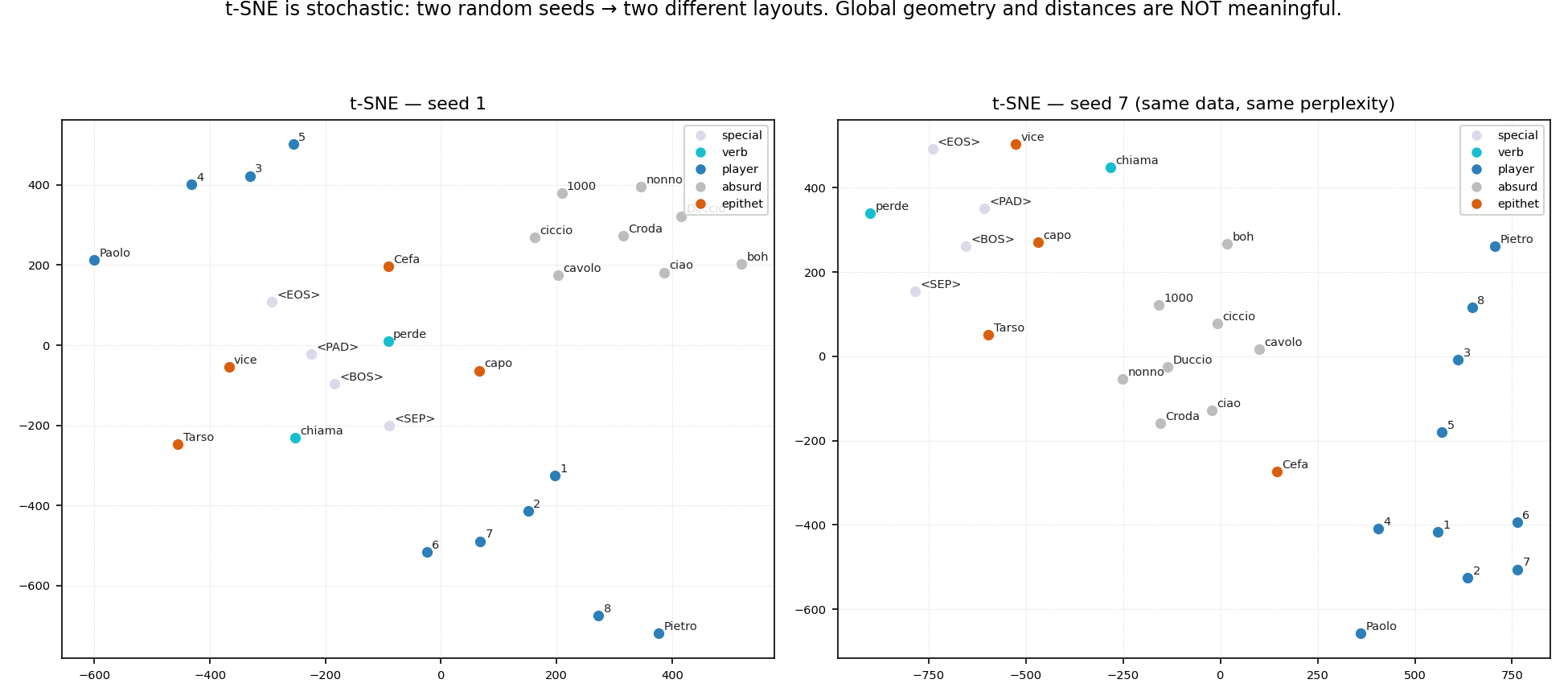
t-SNE seed sensitivity Paolo lands top-left in one run and bottom-centre in the other; the global arrangement reshuffles entirely. If your conclusion would change with the seed, it was never a conclusion about the data.
It is perplexity-sensitive. The one knob (roughly, “how many neighbours count as local”) changes the picture qualitatively; there is no single right value, and small datasets are especially unstable. The classic, still-essential reference is Wattenberg, Viégas & Johnson, “How to Use t-SNE Effectively” (Distill, 2016) — read it before you trust any t-SNE plot, your own included.
Used within its remit — “what clusters with what, locally” — t-SNE is genuinely useful. Read as a map with meaningful axes and distances, it is a confident liar.
5. Capstone — does the intuition survive contact with real language?
Our dialogue game has 28 words and a hand-built rule. Do the same intuitions hold when we scale up to a model trained on something language-like? To check, I took a real TinyStories-trained GPT-2 (segestic/Tinystories-gpt-0.1-3m — a small model trained on the TinyStories corpus of simple children’s stories, with a 50,257-token vocabulary and, conveniently, the same 64-dimensional embeddings as our toy), curated 84 readable whole-word tokens across clear semantic groups (animals, people, nature, colours, verbs, adjectives, function words), and ran the same two unsupervised methods.
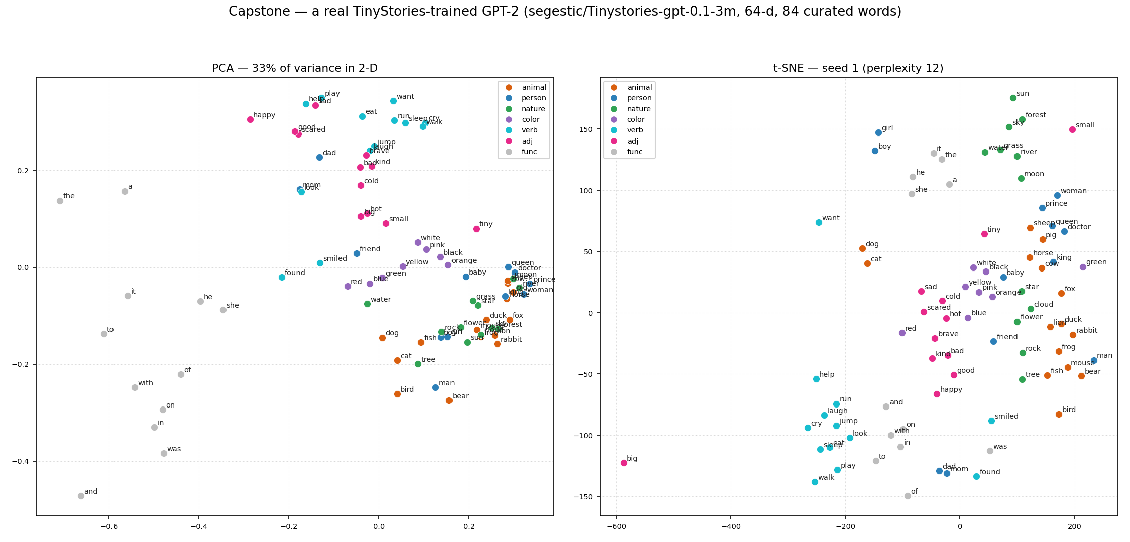
Two things survive the jump to a real corpus. First, the warnings hold: PCA captures only 33% of the variance in 2-D — the same “most of the structure is off-plane” story as the toy — and the function words (grey) peel off along the first PC, a textbook case of frequency dominating the top component (§4b). Second, structure does appear, but softly: in both views you can see animals loosely grouping, function words separating, colours and adjectives drifting together — real, but smeared, not the clean clusters a t-SNE plot’s prettiness might tempt you to over-read. The lesson scales exactly: the maps are useful for orientation, never for measurement, and they get harder to read, not easier, as the model becomes more operationally relevant.
6. How this connects to the rest of the series
This note and its two companions describe one machine from three angles, and they share one matrix:
- The vectors visualised here are the columns of the unembedding matrix W_U that the model scores the final residual against to pick a next token. With tied weights — as in both our toy models — the embedding matrix E and the unembedding W_U = E^\top are the same numbers. So this note is “what the searched dictionary looks like,” and The Final Step is “how the search works.” The maps in §4 are maps of the very dictionary the model’s last step looks words up in.
- The QKV note explains how attention assembles the residual vector that then gets scored. Fig 5 here is the bridge: it watches that residual move through a concept-direction plane built from the embedding rows, and attributes the decisive move to one attention block — the visualization technique of §4a applied to the mechanism of the QKV note.
The through-line: an embedding is a direction in a space the model owns; attention moves the residual through that space; the unembedding searches the space for the nearest word. Visualisation is how we — who cannot see in 768 dimensions — get a partial, question-shaped glimpse of where everything sits.
7. Where this sits in the literature (an honesty box)
None of the findings here are new, and a specialist would recognise every piece; the contribution is expository and the live, perturbable spreadsheet models behind the figures. To locate the material honestly:
- Concept directions and analogies go back to word2vec (Mikolov et al., 2013), whose
king − man + woman ≈ queenis the origin of the whole “linear semantics” picture. That picture is real but partly fragile: later work (Levy & Goldberg; Linzen, 2016) showed the analogies are sensitive to normalisation and to excluding the input words, and are easy to cherry-pick — which is why our in-model analogy landed onlioness, notqueen. - The idea that concepts are linear directions in representation space is the linear representation hypothesis (e.g. Park, Choe & Veitch, 2023, and a long interpretability lineage). That distributed features are packed more than one per dimension is superposition, made precise in Anthropic’s Toy Models of Superposition (Elhage et al., 2022) — the formal version of §2’s lesson and of “single dimensions aren’t interpretable.”
- Does hand-built structure ever help? (the §2 counter-example check.) With care, yes — and none of it rescues hand-wiring. Sparse autoencoders recover monosemantic feature directions from superposition (Bricken et al., Towards Monosemanticity, 2023; Cunningham et al., 2023) — confirming meaning lives in directions, not axes; retrofitting nudges already-learned vectors toward a lexicon to improve them (Faruqui et al., 2015); and the impossibility of unsupervised axis-aligned disentanglement without inductive bias is a theorem (Locatello et al., 2019). Together these say the §2 failure is about dictating and freezing the embedding, not about structure being useless.
- The PCA caveat that top components track frequency/norm rather than clean semantics is well documented; the “delete the top components” fix is All-but-the- Top (Mu & Viswanath, 2018).
- The t-SNE caveats are from van der Maaten & Hinton (2008) and, for practice, Wattenberg, Viégas & Johnson’s How to Use t-SNE Effectively (Distill, 2016); UMAP is McInnes, Healy & Melville (2018), with Coenen & Pearce’s Understanding UMAP as the matching cautionary companion.
- Honesty caveat on the toy: the dialogue-game model is reproduced from the public ToyDialogueGames exercise; the novelty is the transparent, cell-by-cell spreadsheet realisation, the epithet/binding extension, and this exposition for a non-CS audience — not the toy or the methods themselves. The TinyStories capstone uses a community checkpoint (
segestic/Tinystories-gpt-0.1-3m); my own from-scratch TinyStories replication is awaiting hardware.
Appendix A: a Gram-Schmidt projection you can check by hand
Concept-direction maps look like magic but are three dot products. Take a toy 3-dimensional embedding with four words:
king   = ( 2,  1,  0)
queen  = ( 2, -1,  0)
man    = ( 1,  1,  1)
woman  = ( 1, -1,  1)
Suppose we want a “gender” axis and a “royalty” axis. Define them as token differences and build an orthonormal plane.
Axis 1 — gender, as (king − queen):
v1 = king − queen = (0, 2, 0) e1 = v1/‖v1‖ = (0, 1, 0)So e_1 is just the second coordinate. Good: in this toy, dimension 2 happens to carry gender (the male words have +1, the female words −1).
Axis 2 — royalty, as (king − man), then Gram-Schmidt against e_1:
v2  = king − man = (1, 0, -1)
v2·e1 = (1,0,-1)·(0,1,0) = 0          (already orthogonal to e1)
e2  = v2/‖v2‖ = (1, 0, -1)/√2 ≈ (0.71, 0, -0.71)
Project each word onto (e_1, e_2) — two dot products per word:
        e1 (gender)          e2 (royalty)
king    (2,1,0)·e1 =  1      (2,1,0)·e2 = (2−0)/√2 ≈  1.41
queen   (2,-1,0)·e1 = -1     (2,-1,0)·e2 ≈  1.41
man     (1,1,1)·e1 =  1      (1,1,1)·e2 = (1−1)/√2 =  0.00
woman   (1,-1,1)·e1 = -1     (1,-1,1)·e2 =  0.00
Plotted, that is exactly the parallelogram the analogy promises:
   royalty (e2)
   1.41 |  queen ●         ● king
        |
   0.00 |  woman ●         ● man
        +------------------------- gender (e1)
          -1                +1
king − man + woman $= (2,1,0) − (1,1,1) + (1,-1,1) = (2,-1,0) = $ queen, exactly — because we built a space where it works. The sobering content of §2 is that a model trained to predict text does not build such a space for you; it builds whatever predicts best, and the clean parallelogram is the exception, not the rule. Visualisation lets you look for the parallelograms — and, just as importantly, lets you measure how often they are not there.
Appendix B: Glossary
For readers who would like the basics or a refresher. Terms are grouped roughly by where they appear.
Token, vocabulary
A token is the unit of text the model reads — here a whole word; in production models usually a sub-word piece. The vocabulary is the fixed set of all possible tokens (28 in our dialogue game, 50,257 in GPT-2/GPT-3).
Embedding
The vector of real numbers that represents a token. The embedding matrix E has one row per vocabulary token; “looking up” a token means reading its row. The rows are parameters — numbers learned during training — not values fetched from elsewhere (§1).
Encoder (retrieval / vector database)
A separately-trained model that turns a piece of text into one vector so that similar texts get nearby vectors. Used to fill a vector database for semantic search. Examples: OpenAI text-embedding-3, sentence-transformers, ColBERT. It is trained for relevance similarity, a different objective from next-token prediction (§1).
Gradient descent
The training procedure: nudge every parameter a little in the direction that reduces the model’s error, repeat millions of times. It is what “learns” the embeddings.
Residual stream
The running vector the Transformer keeps for each position and updates layer by layer; each attention/MLP block adds its output to it. The model’s prediction is read from the final residual. (See the QKV note.)
Attention head
A sub-mechanism inside a layer that, for each position, decides how much to read from every earlier position. Our toy has 2 layers × 4 heads. “Which head does what” is the central question of mechanistic interpretability.
Logits, softmax
The model’s raw output scores over the vocabulary are logits. Softmax turns them into a probability distribution (exponentiate, then normalise to sum 1).
Tied weights (embedding / unembedding)
Using the same matrix to map tokens→vectors (input) and vectors→token-scores (output, the unembedding W_U = E^\top). Standard for small models; it means the “dictionary” the model searches at the end is the embedding matrix (§6).
Cosine similarity
A measure of how aligned two vectors are: the cosine of the angle between them (+1 = same direction, 0 = orthogonal, −1 = opposite). Ignores length, so it compares direction only.
PCA (Principal Component Analysis)
An unsupervised method that finds the directions along which the data spreads most (the principal components), computed from an eigen-decomposition / SVD of the centred data. Projecting onto the top two gives a 2-D map; the variance explained (e.g. “34.7%”) is the fraction of the data’s total spread those two directions capture — a built-in honesty meter (§4b).
Eigenvector / SVD
The linear-algebra machinery PCA runs on: the singular value decomposition (SVD) factorises the data matrix and hands back the principal directions and how much variance each carries. You do not need the details — just that one svd call yields the PCA axes.
Projection
Mapping high-dimensional points onto a lower-dimensional plane by taking dot products with chosen axes. PCA and concept-direction maps are true projections (the axes keep a fixed meaning); t-SNE is not (§4).
Gram-Schmidt / orthonormal
A recipe for turning two chosen direction vectors into a clean perpendicular (orthonormal) pair of axes, so the two coordinates you read off are independent. Used to build concept-direction planes (§4a, Appendix A).
Concept direction
An axis you choose to stand for a meaning — either a token’s own direction or a difference of tokens (e.g. Paolo − Pietro = “which leader”). Supervised: you bring the meaning (§4a).
t-SNE, UMAP, perplexity
t-SNE and UMAP are nonlinear methods that place points so that local neighbourhoods are preserved, producing cluster-y 2-D pictures. They are not projections: the axes, the distances between clusters, and the global layout carry no meaning, and the result changes with the random seed. Perplexity is t-SNE’s main knob, controlling roughly how many neighbours count as “local” (§4c).
Distributed representation / superposition
Distributed: a concept is carried by a pattern across many dimensions, not one. Superposition: a model packs more feature-directions into a space than it has dimensions, at angles chosen to minimise interference — which is why the axes are not individually meaningful (§2).
Linear representation hypothesis
The empirical idea that many high-level concepts correspond to straight-line directions in representation space — the reason concept-direction maps and analogies (king − man + woman) work at all, when they do (§4a, §7).
Sparse autoencoder (SAE)
A tool that decomposes a model’s activations into many sparse, often human-interpretable feature directions — used to read meaning out of superposition without dictating it in advance (§2, §7).
Ablation
Switching off one component (e.g. one attention head) and re-measuring behaviour, to test what it causally does — as opposed to what its attention pattern looks like. Fig 5’s “which write moved the residual” is the same spirit (§4a; the QKV note’s appendix).
References
Bricken, T., Templeton, A., Batson, J., Chen, B., Jermyn, A., Conerly, T., … Olah, C. (2023). Towards monosemanticity: Decomposing language models with dictionary learning. Transformer Circuits Thread. https://transformer-circuits.pub/2023/monosemantic-features/index.html
Coenen, A., & Pearce, A. (n.d.). Understanding UMAP. Google PAIR. https://pair-code.github.io/understanding-umap/
Cunningham, H., Ewart, A., Riggs, L., Huben, R., & Sharkey, L. (2023). Sparse autoencoders find highly interpretable features in language models. arXiv. https://arxiv.org/abs/2309.08600
Edwards, B. (2012), Drawing on the Right Side of the Brain: The Definitive,, 4th ed, TarcherPerigee.
Elhage, N., Hume, T., Olsson, C., Schiefer, N., Henighan, T., Kravec, S., … Olah, C. (2022). Toy models of superposition. Transformer Circuits Thread. https://transformer-circuits.pub/2022/toy_model/index.html
Faruqui, M., Dodge, J., Jauhar, S. K., Dyer, C., Hovy, E., & Smith, N. A. (2015). Retrofitting word vectors to semantic lexicons. In Proceedings of NAACL-HLT 2015 (pp. 1606–1615). Association for Computational Linguistics. https://arxiv.org/abs/1411.4166
Levy, O., & Goldberg, Y. (2014). Linguistic regularities in sparse and explicit word representations. In Proceedings of the Eighteenth Conference on Computational Natural Language Learning (CoNLL) (pp. 171–180). Association for Computational Linguistics. https://aclanthology.org/W14-1618/
Linzen, T. (2016). Issues in evaluating semantic spaces using word analogies. In Proceedings of the 1st Workshop on Evaluating Vector-Space Representations for NLP (pp. 13–18). Association for Computational Linguistics. https://arxiv.org/abs/1606.07736
Locatello, F., Bauer, S., Lucic, M., Rätsch, G., Gelly, S., Schölkopf, B., & Bachem, O. (2019). Challenging common assumptions in the unsupervised learning of disentangled representations. In Proceedings of the 36th International Conference on Machine Learning (ICML) (pp. 4114–4124). https://arxiv.org/abs/1811.12359
McInnes, L., Healy, J., & Melville, J. (2018). UMAP: Uniform manifold approximation and projection for dimension reduction. arXiv. https://arxiv.org/abs/1802.03426
Mikolov, T., Chen, K., Corrado, G., & Dean, J. (2013). Efficient estimation of word representations in vector space. arXiv. https://arxiv.org/abs/1301.3781
Mu, J., & Viswanath, P. (2018). All-but-the-top: Simple and effective postprocessing for word representations. In International Conference on Learning Representations (ICLR). https://arxiv.org/abs/1702.01417
Park, K., Choe, Y. J., & Veitch, V. (2023). The linear representation hypothesis and the geometry of large language models. arXiv. https://arxiv.org/abs/2311.03658
van der Maaten, L., & Hinton, G. (2008). Visualizing data using t-SNE. Journal of Machine Learning Research, 9(86), 2579–2605. https://jmlr.org/papers/v9/vandermaaten08a.html
Wattenberg, M., Viégas, F., & Johnson, I. (2016). How to use t-SNE effectively. Distill. https://distill.pub/2016/misread-tsne/
Models and tooling behind the figures (all in the julia-impromptu project): the trained dialogue-game model DialogueGame-Tiny-Epithet-Trained.json with its live vocab_map and residual_trajectory reports; the failed hand-wired SemanticTiny.json; the projection pipeline tools/project_embeddings_note.jl (PCA via svd, concept axes via Gram-Schmidt, t-SNE via TSne.jl — one source of truth for every coordinate) and the renderer tools/render_embeddings_note.py.