flowchart LR
    A["query vector<br/>(the final residual)"] -->|"dot product"| B["one score per word<br/>(logits)"]
    B -->|"softmax"| C["probabilities<br/>(the ranking)"]
The Final Step: The Language Model as a Relentless Seeker of the Best Next Word
ABC of LM
LLMs
Transformers
Search
Teaching
The last layer turns all the model’s work into one next word by running a similarity search over the vocabulary. Confidence, sampling, hallucination and tool use all follow from that one dot product. Part 3 of 3.
Third and last in the series “Understanding LLMs to use them better in management and finance.” It closes the loop opened by QKV Attention (how a Transformer moves information between tokens) and Embeddings and the Maps We Draw of Them (where the vectors come from and how to read them). Those two notes built the machinery and the dictionary. This one watches the last step, the moment the model turns all that work into a single next word, and argues that the step is a search. It is written for a reader who is not a computer scientist; the technical terms (logit, softmax, unembedding, …) are collected in the Glossary at the end and explained where first used.
1. The intuition, a relentless search for the next word
Strip a language model down to what it actually does, moment to moment, and it is almost embarrassingly simple. It has a fixed list of possible words, its vocabulary, and at every step it gives each word in that list a score, sorts them, and picks one. Then it appends the chosen word to the text and does the whole thing again, thousands of times over for a single paragraph.
The useful image is a search engine. Generating text is like running a Google search at every step, with two differences. The search runs over the model’s own vocabulary rather than the web, and the query is not typed: it is a vector the model has computed from everything said so far. The results are the whole vocabulary, ranked by how well each word fits as the continuation, and the model reads off the top of the list.
The first two notes were really about the two halves of that sentence. The QKV note showed how the model builds the query: each token is carried forward as a vector (the residual stream), and attention heads and MLP blocks keep modifying it until the last token’s vector encodes everything the model has worked out about what should come next. The embeddings note showed what is being searched: the vocabulary as a cloud of vectors, the dictionary, and how its geometry encodes meaning. This note connects them. The query meets the dictionary, and a word comes out.
2. The mechanism, precisely
After the last layer of the Transformer (Vaswani et al. 2017), the model holds one vector for the final position. Call it h, of length d_{\text{model}}. It is the fully-processed representation of what comes next. To turn it into word scores, the model multiplies it by the unembedding matrix W_U, whose columns are one vector per vocabulary word:
\ell = \tilde h \, W_U, \qquad \ell_i = \tilde h \cdot W_{U}[:,i].
(The tilde is a final LayerNorm that tames the vector’s magnitude first; the glossary has the detail.) The second equation carries the whole note: each score \ell_i, each logit, is the dot product of the model’s query vector with word i’s vector in the dictionary. A dot product is the most basic similarity measure there is: it is large when two vectors point the same way. So the score of a word is how aligned the model’s query is with that word’s entry in the dictionary. Ranking words by their logit is therefore a similarity search over the vocabulary, what the literature calls a maximum-inner-product search.
In the models used here (and in GPT-2 and many others) the embedding and unembedding matrices are tied: W_U = E^\top. The columns the query is scored against are the embedding rows the previous note mapped. The dictionary searched at the end is the dictionary looked up at the start, and the maps in note 2 are maps of the index this search runs over.
The raw logits are then passed through softmax, which exponentiates and normalises them into a probability distribution over the vocabulary. That is the ranked results page, now with percentages. A tiny worked version (three words, by hand) is in Appendix A; the shape of it is all that matters here:
The query did all the hard work; the search itself is a single matrix multiply followed by a normalisation. The search step compares vectors, and performs no reasoning of its own.
3. The search-result page
The worked example throughout is the small word-level Transformer from note 2: two layers, four heads, d_{\text{model}}=64, a 28-word vocabulary, trained on the turn-taking calling game (Pietro chiama Paolo, with epithets that depend on who calls whom). Give it the prompt <BOS> Pietro chiama Paolo and ask for the next word’s ranking:
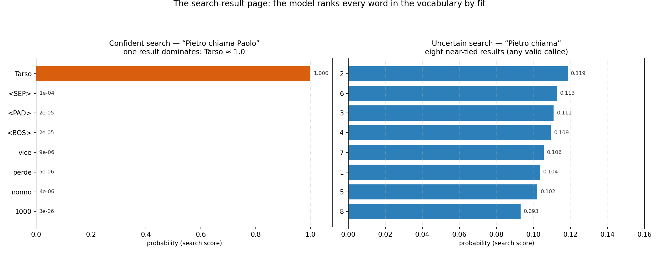
The left panel is the results page for that prompt. The top result is Tarso, the epithet the game’s rule assigns to Paolo when Pietro calls him, with probability 0.9998. Every other word in the vocabulary is down in the one-in-ten-thousand range. That is what a confident search looks like. The query points almost exactly at one entry in the dictionary, and its dot product with that entry is far larger than with any other.
Three properties of that distribution correct the naïve picture of finding the single nearest word:
- A ranking, not one hit. It is a ranking over the whole vocabulary. The model does not retrieve a word; it scores all of them and reports a graded list. Usually the list is informative well below the top.
- Direction says which words, magnitude says how sure. The direction of the query picks out which entries it aligns with; its length controls how peaked the softmax is. A long query makes one word dominate (high confidence); a short one leaves the results flat (high uncertainty). The model’s confidence is encoded in the geometry, not bolted on afterwards.
- Similarity here means trained to fit, not human synonymy. Two words sit close in the dictionary because the model learned they play similar roles in predicting text, which usually looks like meaning but is defined by the training task, exactly as note 2 argued.
4. Confident searches and uncertain ones
Now shorten the prompt to <BOS> Pietro chiama, with the caller named and no callee yet. The right panel above is the result. There is no dominant hit. Instead there are eight near-tied results (the player tokens 2, 6, 3, 4, 7, 1, 5, 8, each around 0.10–0.12), because at this point any valid next player is an equally good continuation. The flat distribution is the model reporting correctly that it does not know which player comes next, only that it must be a player.
Three everyday LLM behaviours follow from that contrast between one tall bar and eight short equal ones:
- Sampling and temperature. When the results are flat, something still has to be chosen. Greedy decoding takes the top bar; sampling rolls a weighted die over the ranking. The standard softmax temperature reshapes the distribution before the roll: high temperature flattens it (more adventurous), low temperature sharpens it (more predictable). Generation is a chain of sampled searches rather than deterministic lookups.
- Hallucination. The search always returns a ranking, even when nothing in the vocabulary genuinely fits. Ask a model for a fact it never learned and the query points nowhere in particular, but the nearest-by-accident words still get scored, softmax still sums to one, and the model still emits its confident-looking top result. A hallucination is a low-quality search the machinery has no choice but to complete. It can be contained: a model can be trained to abstain, calibrated so that a weak hit reads as weak, or grounded in retrieved text so that refusing is an available answer.
- Why prompts and context matter so much. Everything the model knows about this step is compressed into the query vector, and the query is built from the prompt. A better prompt is literally a better search query.
5. How one vector comes to hold a whole world
The query vector h is produced by nothing but multiplications and additions: matrix products, dot products, a normalisation. By the time it reaches the final step, that one short list of numbers has absorbed the meaning of the entire prompt: who is speaking, who was called, what the game’s rule demands, which word is therefore due. Pure numerical manipulation has condensed a whole context into a single point in space.
There is an Archimedean quality to this. Give me a place to stand, and a lever long enough, and I will move the world. The place the model stands is this fulcrum, the last token’s vector. The whole world of the prompt, with all its accumulated context, bears down on that one point, and what it lifts is the next word. The lever is built by the parts the earlier notes described. Attention reaches back across the sentence and binds the relevant tokens into the residual (note 1), and the MLP / feed-forward blocks act, position by position, as a kind of learned lookup table: given “Pietro called Paolo,” they fetch the direction that means “Tarso.” Layer by layer the residual is loaded until it is the long arm of the lever, and the tiny final search is the short arm.
Project the last token’s residual, at each stage of the forward pass, onto a plane built (by the same Gram-Schmidt method as note 2) from two dictionary directions, the epithet Tarso and the callee Paolo:
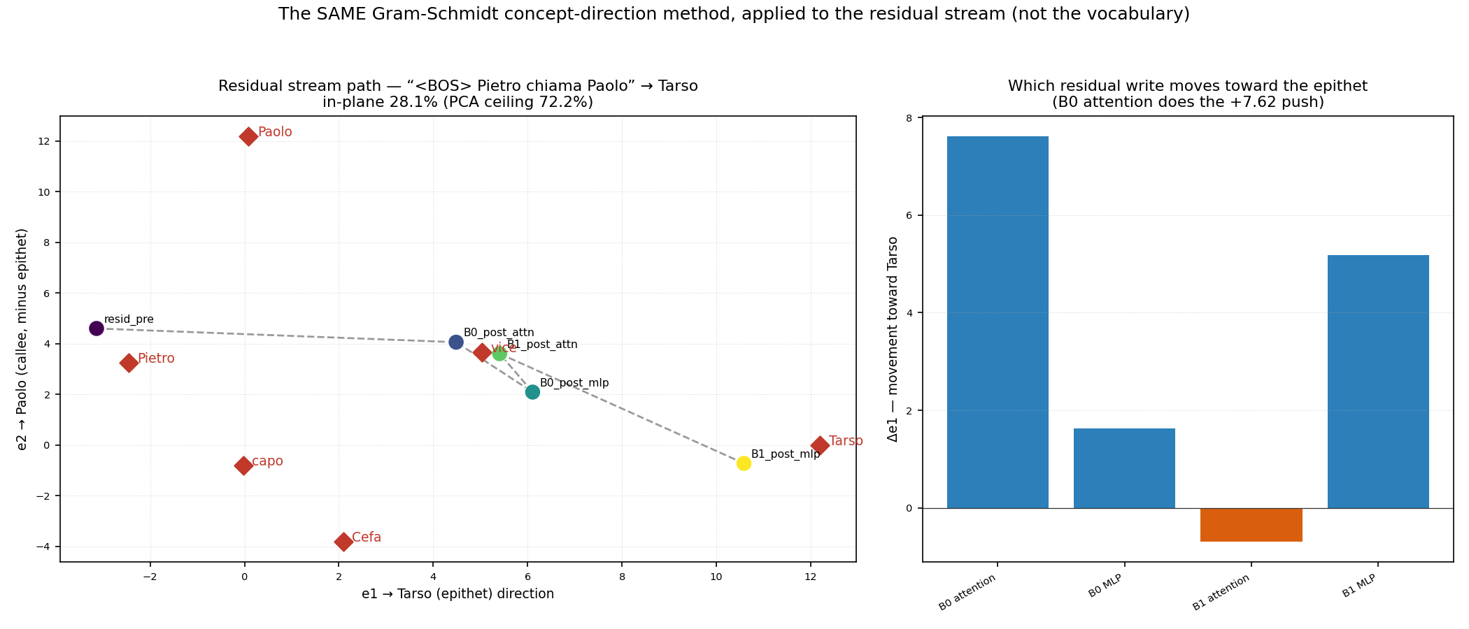
The vector starts near the called name and travels across the plane toward Tarso as the layers run. Its coordinate along the Tarso axis climbs from −3.1 to +10.6, and decomposing the path shows that block-0 attention alone supplies +7.62 of that push. Moving the residual toward a word’s direction is raising that word’s logit (tied weights again), so this picture is the search ranking being rewritten as the forward pass proceeds. Read as rankings rather than geometry, the same thing is the logit lens: the unembedding applied at each intermediate stage, to see what the model would predict if it had to commit there.
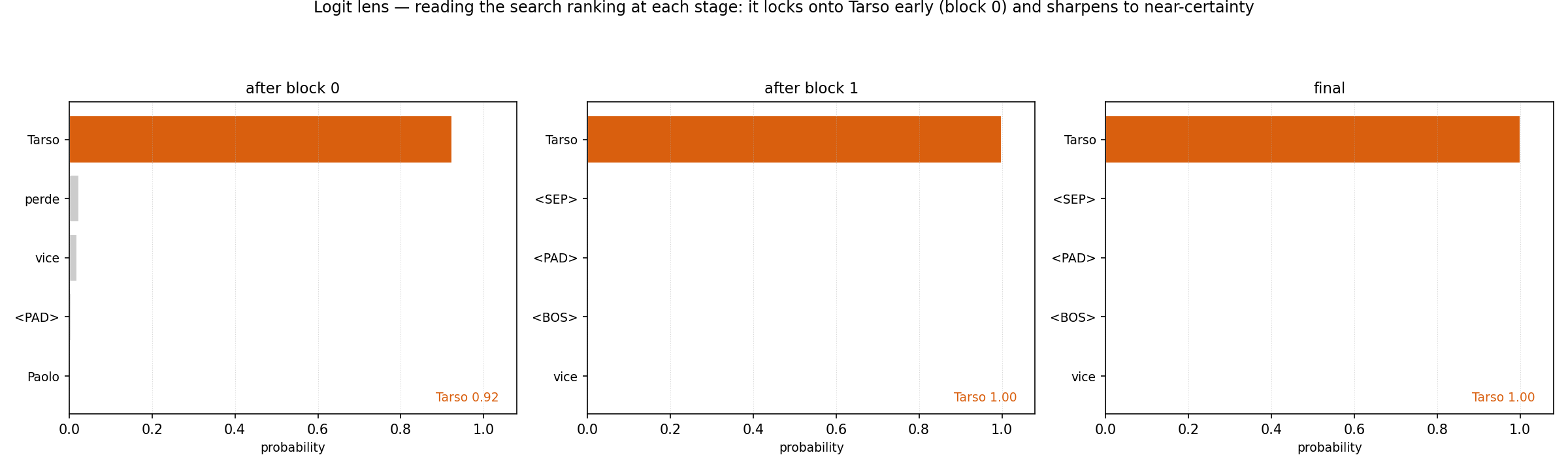
By the end of the first block the search already ranks Tarso top (0.92); the second block sharpens it to near-certainty. The decisive work happens early on this prompt, where the trajectory said it did. The mechanism is binding, then lookup, then a dot product, and that is enough to make a vector carry a world.
6. From a toy to a thousand-page contract
It would be fair to object that lifting the word “Tarso” out of a 28-word vocabulary is a parlour trick. The machinery of the output layer is identical at the top of the field. Base transformer models do what the toy here does: score every word in the vocabulary by dot product with a computed query, softmax, sample, append, repeat. A production system wraps more exotic parts around the output layer (speculative decoding, constrained decoding, MoE routing, RLHF-tuned sampling). What differs is scale: a query vector of 12,288 numbers instead of 64 (note 2), a dictionary of 50,000-plus word-pieces instead of 28, and a lever built from dozens of layers trained on a sizeable fraction of the written internet.
From that loop of ranking the vocabulary and picking a word comes the entire observed richness: a comedy sketch with a setup and a punchline, a sonnet that scans, a scientific paper with a coherent argument, an investor report that ties its narrative to its numbers, a full contract with cross-referencing clauses. Each of those is produced one next-word search at a time, each search standing on the fulcrum the previous words built. What is remarkable about large language models is that this, at scale, is enough.
7. Tools, search and code
Modern systems add one more move, the one that turns a text generator into an assistant. The find-next-word loop is orchestrated with real outside power: a web search, a calculator, a code interpreter, or other applications reached through MCP servers. It is tempting to imagine the model using these tools the way a person does. What happens is simpler than that.
Picture the prompt as a conveyor belt of text that the model endlessly reads and extends. When a tool is involved, the model does not leave the belt to operate machinery. It writes onto the belt a request, a few tokens that mean “search the web for X” or “run this code.” An external harness, sitting outside the model, notices that text, performs the actual action, and lays the result back onto the belt as more text: the search snippets, the computed number, the program’s output. Then the same next-word loop resumes, now reading a context enriched with fresh, grounded material. The tool’s answer is not stored in some special memory; it becomes ordinary prompt text, indistinguishable in kind from what the user typed.
Designs of this kind sit on the Transformer’s natural evolution path and are widely in use; MCP is a popular example. Modern systems that reach for higher performance bypass the belt: the harness sits inside the serving loop, or native tool tokens are triggered.
The lever’s world, the context pressing on the query, is therefore no longer limited to what the user wrote and what the model already knew. It can now include this morning’s web page, an exact calculation, the output of a freshly compiled program. The mechanism underneath never changes: every one of those additions is more text on the belt, and every word the system produces is still one dot-product search over the vocabulary. Where the belt is the interface, an agent’s capability comes from what gets written onto it, and from a search that keeps reading.
8. Where this sits, and where the analogy breaks
Nothing in the mechanism here is a new finding; a specialist would recognise every piece. That the unembedding is a dot-product readout that can even be applied to intermediate layers is the logit lens (nostalgebraist; rethought as the tuned lens, Belrose et al. 2023). That the feed-forward blocks behave like a lookup table is Transformer Feed-Forward Layers Are Key-Value Memories (Geva et al. 2021). The output-layer-as-similarity-search idea goes back to the neural probabilistic language model of Bengio et al. (2003) and to word2vec (Mikolov et al. 2013). The pedagogy of doing the whole thing transparently has been done before too: Ishan Anand’s Spreadsheets Are All You Need is a proof that GPT-2 can be implemented in a spreadsheet. The contribution here is only the exposition for a non-technical audience and the live, perturbable toy behind the figures; the toy game itself is reproduced from the public ToyDialogueGames exercise.
The search-engine image earns its keep but must not be pushed too far. It breaks in four places:
- There is no external corpus. A web search ranks billions of documents; this search ranks only the model’s own fixed vocabulary (tens of thousands of word pieces). It cannot return anything that is not already a token.
- The query is computed, not typed. All the work, and all the cleverness, is in constructing the query vector. The search step itself is a trivial linear operation. “It’s just doing search” is true and deeply misleading at once: the search step is trivial, and the query is where the model is.
- It returns a distribution and then gambles. Unlike a search box that shows a fixed list, generation samples from the ranking, so the same prompt can yield different continuations. Determinism is a special case of the decoding step (temperature zero), not the default. Even at temperature zero a served model is not bit-reproducible (batching reorders the arithmetic).
- Relevance is the training objective. A word scores high because the model was trained to make the right next token score high, which approximates meaning but is not the same thing, and is exactly why the results can be fluent and wrong together.
That last point connects back to the second note. A vector database (the engine of retrieval-augmented generation) also performs a similarity search, but over an external corpus, using a query produced by a separately trained encoder. A language model performs a similarity search over its own vocabulary, using a query it computes internally. The operation is the same; the index and the source of the query differ. RAG, seen this way, is a way to put better text on the conveyor belt: it drops genuinely relevant documents into the context so that the model’s computed query, and therefore its next-word search, points somewhere grounded.
9. What this means for using LLMs in management and finance
One mental model is worth carrying away from these three notes. A language model is not a database queried for facts, and not a mind that knows things. It is a machine that, at every step, draws on the knowledge compressed into its weights to build a vector summarising the context, and then runs a similarity search over its own vocabulary for the best next word. Run that step again and again and an articulated response takes shape, one word at a time.
What comes out is unlike the result of a database query. It is not a selection of pre-baked text or data retrieved from a store; it is closer to a kind of mechanical expert judgement, a chain of small inferences over knowledge the model has metabolised from training on many similar cases.
Four consequences follow in practice:
- Hallucinations. They are not malfunctions; they are the search completing when it shouldn’t. The remedy is to improve the query, by putting the right facts on the conveyor belt (RAG, tools, better context).
- Prompting is query construction. Time spent shaping the context is time spent aiming the search. Prompting is the highest-leverage thing a non-technical user controls.
- Confidence is readable. A small base model that is sure has a peaked distribution; a flat one is a warning. Where a system exposes token probabilities or lets you vary temperature, those are direct windows onto how strong the search hit was in that model.
- Tools extend the world the model can lift, not the mechanism. Web search, a calculator, a code runner, an MCP-connected application: each one enriches the text the next-word search reads. Understanding that boundary is what lets you reason about what these systems can and cannot reliably do.
The model is a relentless seeker of the best next word. The poems, the reports, the contracts and the agentic tool use are what that one search becomes when it stands on a rich enough world and is run, patiently, again and again.
Appendix A, the search by hand
Take a deliberately tiny model: a query vector of length 3 and a three-word vocabulary, each word a row of the (tied) dictionary.
A caveat on what is being skipped, so the example is not mistaken for the whole machine. In a real run there is a prompt, text such as <BOS> Pietro chiama Paolo, and a query-building mechanism: the embedding lookup, the attention blocks, and the MLP blocks of Notes 1 and 2, which between them read the prompt and grind it down into the single final-residual vector h. All of that is the hard, interesting part. Here the finished h and a three-word dictionary are simply posited, so that the search step itself, dot product then softmax, stands alone and can be checked by hand. Read the numbers below as a supposition: the upstream layers handed over this query against this dictionary.
query  h     = ( 1.0,  0.5, -0.2)        the final residual

dictionary:
   Tarso      = ( 1.2,  0.4, -0.1)
   Cefa       = ( 0.3,  1.0,  0.2)
   Paolo      = (-0.5,  0.2,  0.9)
Score each word, a dot product with the query (this is the search):
ℓ(Tarso) = 1.0·1.2 + 0.5·0.4 + (-0.2)(-0.1) =  1.20 + 0.20 + 0.02 =  1.42
ℓ(Cefa)  = 1.0·0.3 + 0.5·1.0 + (-0.2)( 0.2) =  0.30 + 0.50 − 0.04 =  0.76
ℓ(Paolo) = 1.0(-0.5)+ 0.5·0.2 + (-0.2)( 0.9) = −0.50 + 0.10 − 0.18 = −0.58
Softmax, turning scores into a ranked probability list:
exp:   e^1.42 = 4.14,   e^0.76 = 2.14,   e^-0.58 = 0.56     sum = 6.84
prob:  Tarso 4.14/6.84 = 0.61    Cefa 0.31    Paolo 0.08
Tarso wins, because its dictionary entry points most nearly the same way as the query. The dot products are the search; softmax only turns the scores into a tidy ranking. Make the query longer (multiply h by 3, keeping its direction) and the logits become (4.26, 2.28, -1.74) with probabilities (0.87, 0.12, 0.01): the same winner, sharper confidence. Direction chose the word; magnitude set the certainty.
Appendix B, Glossary
Continues the glossary of note 2; here are the terms specific to the final step.
Logit
A word’s raw, unnormalised score, the dot product of the model’s query vector with that word’s dictionary entry. One logit per vocabulary word.
Softmax
The function that turns a vector of logits into a probability distribution: exponentiate each, divide by the total. Bigger logits become bigger probabilities; the result sums to 1.
Unembedding
The matrix W_U that maps the final vector to one logit per word. Its columns are word vectors. With tied weights it is the transpose of the embedding matrix, the same dictionary used for input lookup and output scoring.
Maximum-inner-product search (MIPS)
Find the items whose vectors have the largest dot product with a query. Ranking the vocabulary by logit is exactly this, a similarity search with the dot product as the similarity.
Logit lens
A diagnostic: apply the unembedding to the residual at an intermediate layer to see what the model would predict if forced to commit there. It works because the residual lives, throughout the network, in the space the final readout uses, provided corrections for scale drift are applied, as in the tuned lens.
Key-value memory (feed-forward block)
A way of reading the MLP/feed-forward sub-layers: each behaves like a stored key–value pair, recognising a pattern in the residual (“Pietro called Paolo”) and writing an associated direction back (“toward Tarso”). These are the model’s per-token lookups.
Greedy decoding, sampling, temperature, top-k / top-p
Ways to pick a word from the ranked distribution. Greedy takes the top one. Sampling draws at random in proportion to probability. Temperature rescales the distribution before drawing: high = flatter/more varied, low = sharper/more predictable. Top-k / top-p restrict the draw to the most probable words.
RAG (retrieval-augmented generation)
Fetching relevant documents from an external store (via a vector-database similarity search) and inserting them into the prompt, so the model’s next-word search runs over a context grounded in real text.
MCP (Model Context Protocol)
A standard by which a model’s host application connects to external tools and data sources. It is client–server: the host application runs the client, and each tool or data source is exposed by a server. In the picture of this note: a way for results computed outside the model to be written back onto the prompt conveyor belt as text the next-word loop then reads.
References
Anand, I. (2024). Spreadsheets are all you need: A spreadsheet implementation of GPT-2. https://spreadsheets-are-all-you-need.ai/
Belrose, N., Furman, Z., Smith, L., Halawi, D., Ostrovsky, I., McKinney, L., Biderman, S., & Steinhardt, J. (2023). Eliciting latent predictions from transformers with the tuned lens. arXiv. https://arxiv.org/abs/2303.08112
Bengio, Y., Ducharme, R., Vincent, P., & Jauvin, C. (2003). A neural probabilistic language model. Journal of Machine Learning Research, 3, 1137–1155. https://www.jmlr.org/papers/v3/bengio03a.html
Geva, M., Schuster, R., Berant, J., & Levy, O. (2021). Transformer feed-forward layers are key-value memories. In Proceedings of the 2021 Conference on Empirical Methods in Natural Language Processing (EMNLP) (pp. 5484–5495). Association for Computational Linguistics. https://arxiv.org/abs/2012.14913
Mikolov, T., Chen, K., Corrado, G., & Dean, J. (2013). Efficient estimation of word representations in vector space. arXiv. https://arxiv.org/abs/1301.3781
nostalgebraist. (2020, August 31). Interpreting GPT: The logit lens. LessWrong. https://www.lesswrong.com/posts/AcKRB8wDpdaN6v6ru/interpreting-gpt-the-logit-lens
Vaswani, A., Shazeer, N., Parmar, N., Uszkoreit, J., Jones, L., Gomez, A. N., … Polosukhin, I. (2017). Attention is all you need. Advances in Neural Information Processing Systems, 30. https://arxiv.org/abs/1706.03762
Models and tooling behind the figures (in the julia-impromptu project): the trained dialogue-game model DialogueGame-Tiny-Epithet-Trained.json, whose Forward_TopK ranking and logit-lens recompute live as you edit the prompt; the series’ live companion EmbeddingAtlas.json, whose final_step_search report shows the confident/uncertain search pages and the logit-lens locking on; the figure data computed bundle-pure in tools/compute_note3.jl and rendered by tools/render_note3.py. The residual-trajectory figure is reused from note 2.