Forecasting a company’s accounts and cash flow with an AI assistant
Episode 1 of the AI-assisted financial analysis series. I open a half-built leveraged-buyout model, type a few numbers, write four formulas by hand, and then describe in ordinary English what the income statement, the balance sheet and the cash-flow statement should do. An AI assistant writes the rest. The three statements depend on each other in a circle, and the engine solves the circle with no setting to turn on. This post is the canonical write-up. The video below is the twelve-minute version, and everything here is readable on its own. New readers may want the launch manifesto first; readers who want to know what is running should see Impromptu under the hood.
The bench, in one minute
Three things are on the bench in this episode.
The Workbench is this site: field notes from an ongoing experiment in building small, transparent tools for teaching finance and for probing how AI works. The blog is the permanent home; the videos are demonstrations.
Impromptu is the modeling engine on screen. It is a multidimensional spreadsheet in the tradition of Lotus Improv, a tradition that continues in Quantrix Modeler, the tool of our Financial Planning Lab at Trento. In a multidimensional spreadsheet there is no =B7*C7 to drag down a column. The formula is Gross Profit = Sales + Raw Materials + Direct Labor Costs, written once over a whole named array, and it applies to every year at once. The formula says what it means. Impromptu is a research prototype, not a product and not a replacement for the tools we teach with. It exists because some questions can only be answered with an instrument that can be taken apart. Its architecture (a Julia computation server, an Elm browser client, a formula language that compiles to Julia) is the subject of a separate note.
Claude Code is the AI assistant. It is wired to the live engine rather than reading screenshots of the model: it is connected through MCP (the Model Context Protocol), a standard way for an AI’s host application to reach external tools. Claude can list the datasets, read the existing formulas, write new ones, trigger a recalculation and read the results back, while I watch every step on screen. When Claude writes a formula, that formula lands in the model the way mine does, in the same language, and I can read it afterwards.
Technical terms are named where they first appear and collected in the glossary at the end. The complete formula set is in Appendix A, so a reader can rebuild the model in the tool of their choice.
The company is a small manufacturer, bought in a leveraged buyout at the end of 2022 for 196,000 (thousands, throughout), financed with 90,000 of bank debt and 106,000 of sponsor equity. We have 2022 actuals and we want the next four years: what the accounts look like, and where the cash goes.
1. A model is a graph of small matrices
The first surprise for a spreadsheet user is that there is no sheet. There is a list of datasets in the left-hand tree, and each dataset is a small matrix with named axes.
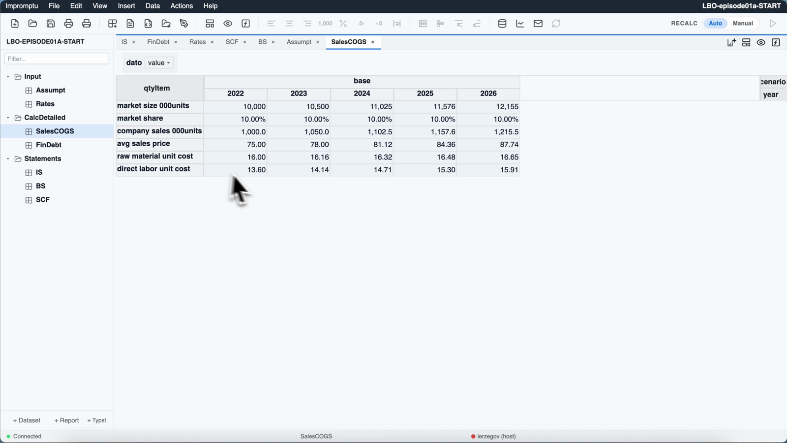
SalesCOGS, a matrix whose axes are the six quantity/price line items and the five years.
Each axis is a dimension, and its labels are coordinates. The SalesCOGS dataset in Figure 1 has three dimensions: qtyItem (six coordinates: market size, market share, company sales, average price, and two unit costs), year (2022 through 2026), and scenario (just base today; that axis will hold the what-if cases).
The difference from Excel is here. In a sheet the line items of the income statement are rows that contain formulas. In Impromptu they are coordinates of a dimension called ISitem, and the dataset holds one formula per coordinate. Gross Profit is a name the engine knows, not cell B7. Impromptu calls a dimension used this way a coord-formula dimension. This is the Improv idea: the structure of the statement is data, and the formulas attach to that structure by name.
Because the numbers and their labels are the same object, the grid can be re-pivoted freely. Dragging year out of the columns and into the page tray shows one year at a time. The model and the formulas are unchanged, and nothing is retyped.
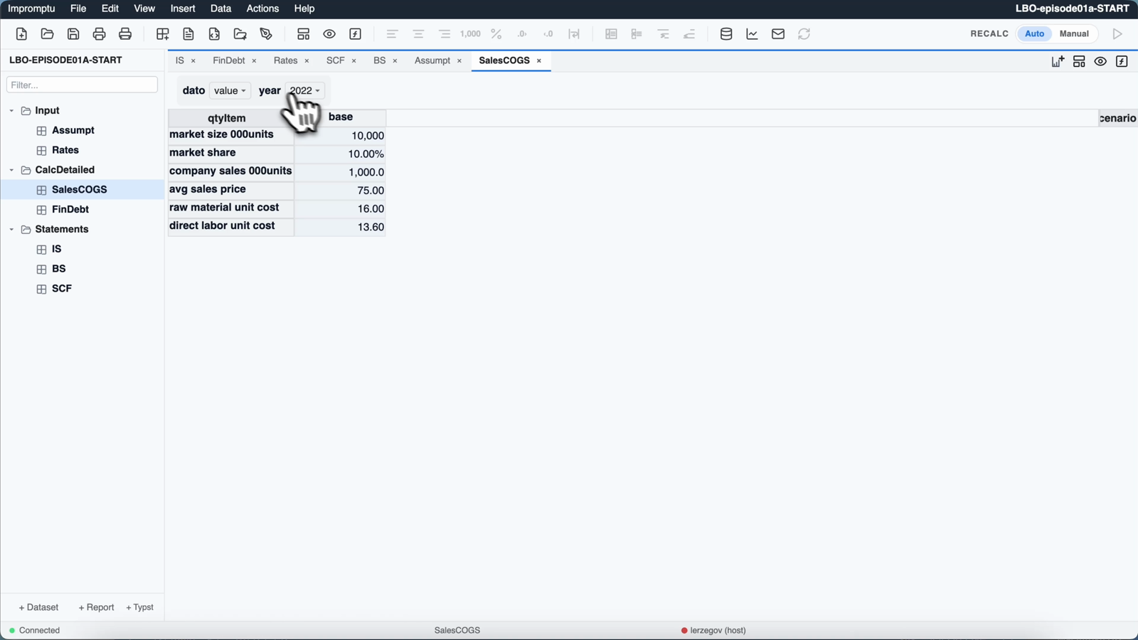
year has been dragged into the page tray at the top, so the grid now shows a single year and the years become a selector. No formula was touched.
The datasets on screen are of two kinds. Four are already wired and we will not touch them: Assumpt (every input assumption, in collapsible groups), Rates (tax rate 35%, cost of debt 6%), SalesCOGS (a driver-led forecast: market size grows 5% a year, our share holds at 10%, average price grows 4%), and FinDebt (a debt schedule we are about to fill in). Three are empty skeletons, and building them is the work of the episode: IS, BS and SCF, the income statement, the balance sheet and the statement of cash flows.
The skeletons have all their structure: every dimension, every line-item coordinate, every group. They have no formulas. That is deliberate: on camera we fill a skeleton rather than draw one.
2. A little by hand
Before delegating anything, I want to show that the tool is learnable: a person can sit down and drive it. I type some numbers and write four formulas, each chosen to teach one move.
The numbers first. The debt in this deal is pre-determined, so I type the five outstanding balances straight into FinDebt: 90,000 at the close, rising to 100,000 in 2024, then amortizing slightly to 99,000. In Assumpt I fill the five working-capital drivers, the ones a credit analyst recognizes on sight: 60 days of receivables, 30 days of raw materials, 45 days of finished goods, 15 days of wages payable, 45 days of other payables.
M1, last year’s value and another dataset
Interest is last year’s debt times the cost of debt. In the formula editor I type Interest =, then click the Outstanding debt cell rather than typing its name. The editor writes the reference for me. Then I add the positional operator by hand:
Interest = Outstanding debt[year:prev] * Rates.cost of debt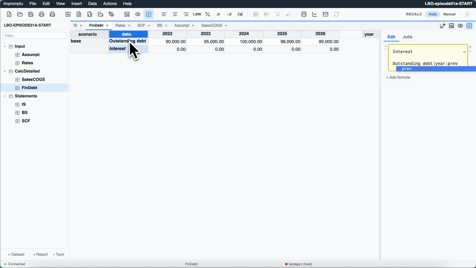
year is marked as a recursive dimension, so the editor offers first, prev, rest inside the brackets, the vocabulary of a roll-forward. Tab accepts.
The formula carries two ideas. [year:prev] means the value of this line in the previous year. That vocabulary comes from marking year as a recursive dimension, and it is how every roll-forward in this model is written. Rates.cost of debt reaches into a different dataset by name. The model is a graph of small matrices that read each other, not one enormous sheet.
When I confirm, the whole row computes, because the debt is already there: 5,400 in 2023, then 5,700, 6,000 and 5,880. One formula covers five years.
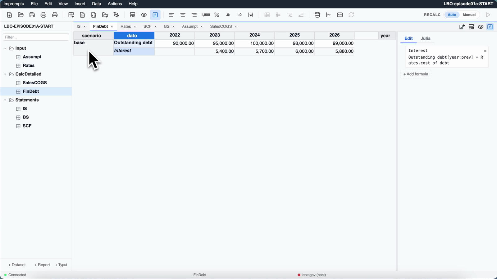
M2, a formula written by name
Next the income statement, and the pure Improv move:
Gross Profit = Sales + Raw Materials + Direct Labor CostsI never touch a cell reference. I click the line-item headers, and because those line items are coordinates, the formula is a sentence about the statement. It applies across all five years at once.
It shows blank, because Sales, Raw Materials and Direct Labor Costs do not exist yet. It fills in once they do, in the next section.
One convention matters for every subtotal in this model: costs are carried as negative numbers. Raw Materials in 2022 is −16,000, not 16,000. Every subtotal is then a plain sum, with no minus signs to remember and no sign errors buried three levels down.
M3 and M4, a working-capital driver and a subtotal
Two lines on the balance sheet. Receivables are the classic days-based driver, and again the reference crosses datasets:
accounts receivable = (Assumpt.AR days * IS.Sales) / 365Then the subtotal. The balance-sheet line items are organized into a collapsible hierarchy: Assets contains a NWC group containing receivables, inventories and payables. Impromptu can add up a group by name:
Net working capital = sum_group(NWC)That is 12,328.8 + 1,315.1 + 3,649.3 − 1,237.0 − 3,180.8 = 12,875.3 in 2022, and it stays correct if I ever add a line to the group. Collapsing NWC in the grid leaves a single subtotal row.
The balance sheet also carries two value layers over the same axes, which Impromptu calls arrays. value is the balance, and delta is the year-on-year change, defined once for the whole dataset:
delta = value - value[year:prev]The cash-flow statement will read those changes. This is the second thing a multidimensional spreadsheet has that a grid of cells does not: a dataset is a stack of typed layers rather than a single sheet of numbers.
Four formulas, in about three minutes, are the whole manual lesson. Everything else in this model is the same four ideas repeated.
3. Handing the modeling to Claude
The income statement has thirteen line items and one formula. Instead of typing the other twelve, I describe what the statement should do:
The
ISdataset has all its line-item coordinates; I have already inserted a formula for one line (Gross Profit); it’s recursive onyear, base scenario. Complete the income statement, 2022→2026. 2022 is actuals — the… t0figures inAssumpt. From 2023 on, drive it off the forecast: revenue = units × price fromSalesCOGS; raw-material and direct-labour costs = the same volumes × the unit costs; sales-&-marketing and administrative = theirAssumptpercentage of sales. Then EBITDA, depreciation (from the balance sheet’sDepreciationline), EBIT, interest (fromFinDebt), pre-tax income, tax at theRatestax rate, net income. Keep costs negative so every subtotal is a plain sum.
The prompt is a description rather than a list of formulas, the one a finance lecturer would give a class: the functional content of an income statement, in the order the statement runs, plus the two conventions that are local to this model (costs negative; 2022 comes from the actuals).
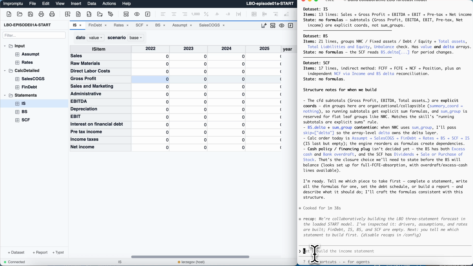
Claude inspects the model first: the datasets, the dimensions, which coordinates exist, and what the one existing formula looks like, so that it can match the style. Then it writes the statement.
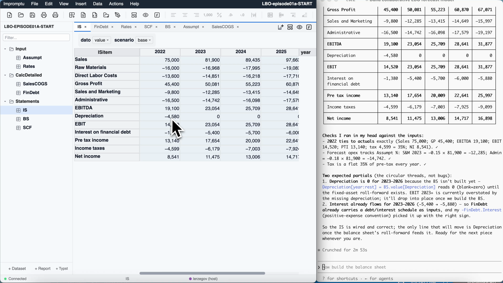
Gross Profit line I wrote by hand three minutes ago is now filled in, because its inputs exist. In the right pane Claude checks its own work against the 2022 actuals and flags the two lines that are still zero.
Two things happen here. The first follows from the coordinate idea. I wrote Gross Profit when Sales was nothing but a label. Now Sales has a formula, and my line fills in. I never went back to it. The formula was always a statement about the structure; it had nothing to read.
The second is a loose end. The income statement is complete but not yet true. Depreciation in Figure 6 reads −4,580 in 2022 (an actual) and zero thereafter. It is zero because I asked for depreciation to come from the balance sheet’s Depreciation line, and there is no balance sheet yet. So 2023 EBIT reads 23,054 where it should read 17,433, and net income reads 11,475 where it will settle at 7,821.
That is the first strand of a circular system, still unconnected. Claude noticed it unprompted and said so: it named the two “expected partials” and predicted exactly which lines would move once the balance sheet arrived.
4. The rest of the balance sheet, and the cash flow
The next ask is the bulk of the model, and it goes out in one prompt: finish the operating side of the balance sheet (no financing yet), and build the whole cash-flow statement.
The balance sheet’s operating side is two ideas. The remaining working-capital lines follow the same days-basis as the receivables I wrote by hand: inventories driven by materials and labour cost, payables by labour and admin, and by materials and marketing. The fixed assets are a roll-forward:
Capital expenditures[year:rest] = Assumpt.capex pct of sales change * (IS.Sales - IS.Sales[year:prev])
Depreciation[year:rest]         = -(Assumpt.avg depreciation on NFA) * (Net fixed assets[year:prev] + Capital expenditures)
Net fixed assets[year:rest]     = Net fixed assets[year:prev] + Capital expenditures + Depreciation
The middle line is where the loop closes. The rate is an average rate applied to the net asset base, last year’s net fixed assets plus this year’s capex, not the statutory rate a tax code applies to an asset’s gross cost. That base depends on capex; capex depends on the increase in sales; sales are in the income statement; and the income statement subtracts this depreciation. The model now goes around in a circle, on purpose.
The cash flow is the indirect method, built from the income statement, the balance sheet’s delta layer, and the debt schedule. The statement starts from EBIT, taxes it as if the firm had no debt, adds back depreciation (a non-cash charge), and subtracts the cash absorbed by working capital and by capex. That is FCFF, the free cash flow to the firm: 9,660 in 2023. Adding net borrowing and subtracting the after-tax interest the debt costs gives FCFE, the free cash flow to equity: 11,150 in 2023.
Then a modeling decision, which is the reason this model closes without a solver:
Dividends[year:rest]                = ifelse(FCFE>0, -FCFE, 0)
Sale or Purchase of Stock[year:rest] = ifelse(FCFE<0, -FCFE, 0)
NCF[year:rest]                       = FCFE + Dividends + Sale or Purchase of Stock
Every year’s free cash flow to equity is fully absorbed. If it is positive it goes out as a dividend; if it is negative the sponsor covers it with a stock issue. Net cash flow is therefore zero every year, and cash stays at 16,500. The Excess cash and Bank overdraft lines are wired, but in this base case they never move.
This is a modeling choice, not a rule of accounting. A real LBO model would define a dividend and cash-reserve policy, and the cash balance would normally change from year to year. Here I want the cleanest demonstration of a circular system converging, so I fix the cash policy and let the equity account absorb everything. Relaxing the absorption rule would make the residual reappear as excess cash or an overdraft, which is what those two lines are for, in a later episode.
At this point the balance sheet has assets and no equity. It does not balance, and Claude says so.
5. Closing the circular loop
One more ask: make it balance.
There are three moves. Pull cash and the financing flows over from the cash-flow statement. Set the opening equity to the sponsor’s cheque, the purchase price net of the debt drawn:
Sale or Purchase of Stock[year:first] = Assumpt.equity purchase price - Financial debtThat is 196,000 − 90,000 = 106,000. Then stockholders’ equity rolls forward as opening balance, plus net income, minus dividends, plus any stock issued:
Stockholders Equity[year:first] = Sale or Purchase of Stock
Stockholders Equity[year:rest]  = Stockholders Equity[year:prev] + Net Income + Dividends + Sale or Purchase of Stock
For 2023 that reads 106,000 + 7,821 − 11,150 = 102,672. The company is profitable and its equity falls, because it pays out more than it earns, which is the LBO in one line.
Finally the plug. At the close, the sponsor paid 196,000 for a business whose identifiable net operating assets are worth 62,875 and which holds 16,500 of cash. The difference is goodwill:
Goodwill[year:first] = (Financial debt + Bank overdraft + Stockholders Equity) - (Total net operating assets + Excess cash)
Goodwill[year:rest]  = Goodwill[year:prev]
which comes to 196,000 − 62,875 − 16,500 = 116,625, carried forward unchanged. The last three lines are Total assets, Total Liabilities and Equity, and a check line, Unbalance, the difference between them.
The dependencies run in circles. Depreciation runs from the balance sheet into the income statement. Net income runs from the income statement into the balance sheet’s equity. The cash-flow statement reads both, and its dividends and stock issues run back into the equity roll-forward, while its cash lands on the balance sheet. The three statements are a simultaneous system: none of them can be computed before the other two.
In a conventional spreadsheet this is the moment to find the iterative-calculation setting, or to break the loop by hand with a lagged variable. Impromptu does neither. When the model is loaded, the engine works out the dependency order of the datasets, finds that IS, BS and SCF form a cycle group, and iterates that group to a fixed point: up to 100 passes, stopping when nothing moves by more than one part in ten billion. There is no switch to enable and no circular-reference warning. The circularity is a property of the accounting, and the engine treats it as one.
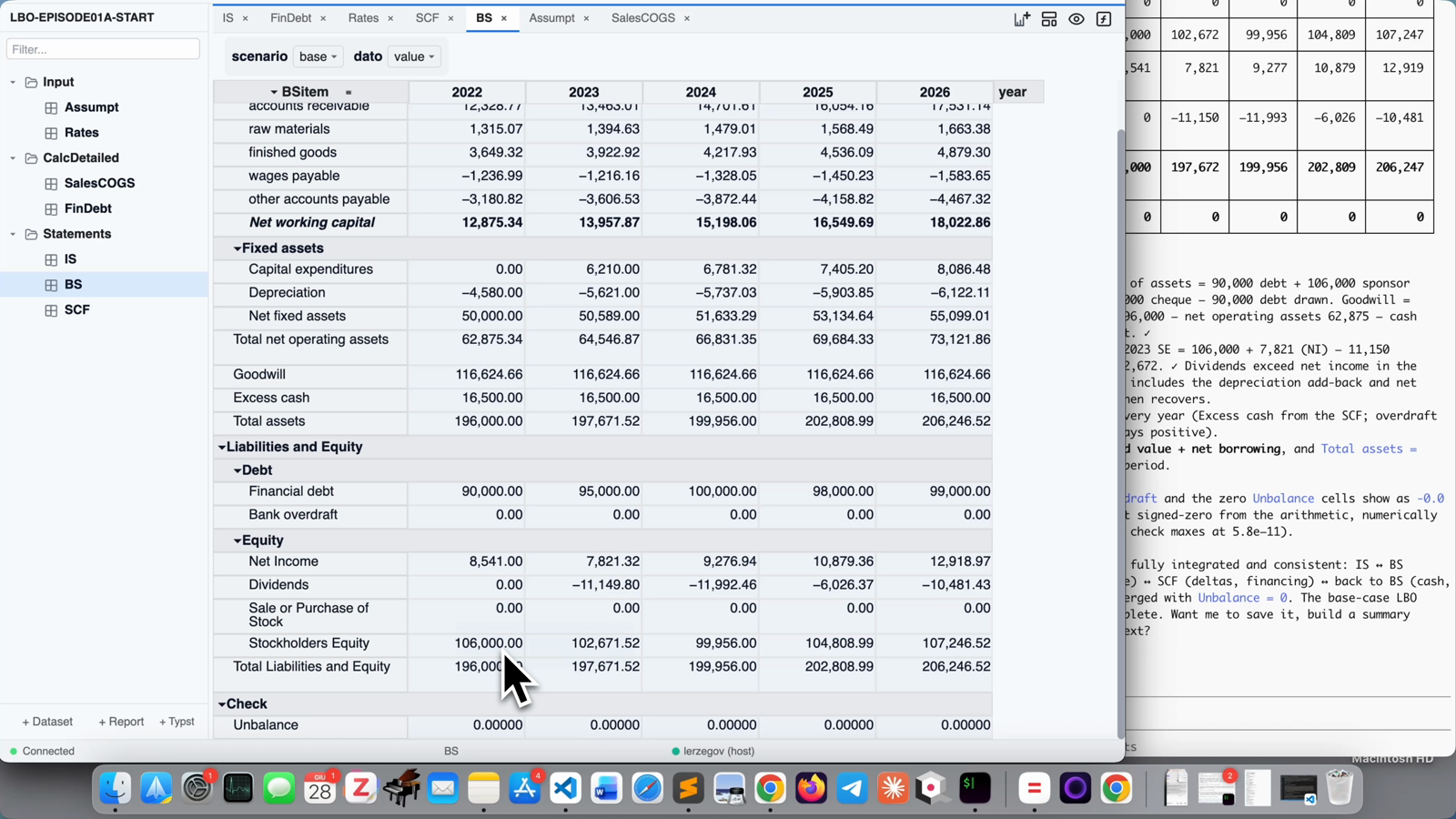
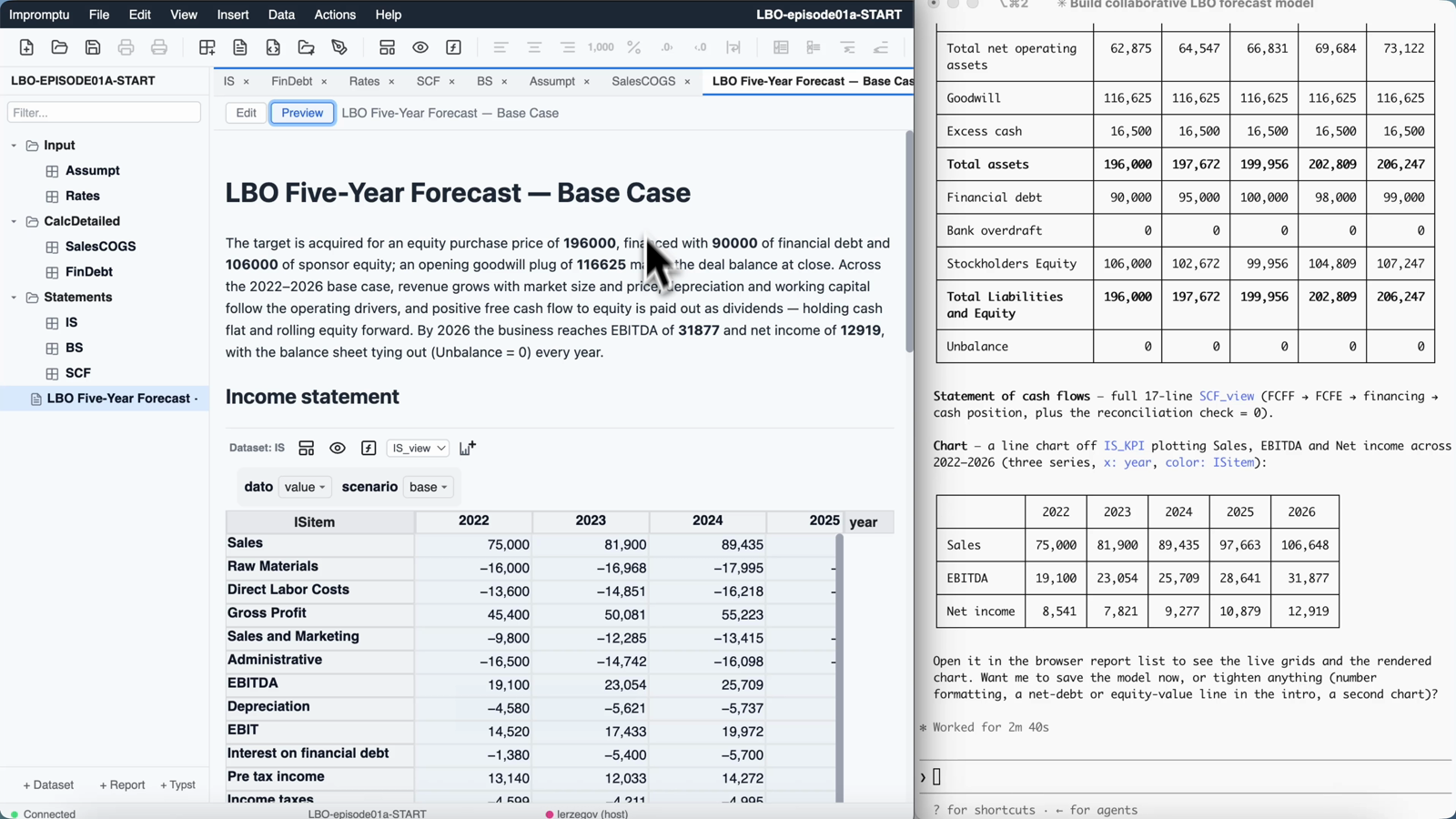
Unbalance reads 0.00000 for every year. Assets of 196,000 at the close grow to 206,247 by 2026. Stockholders’ equity dips: 106,000 at the close, down to 99,956 by 2024 as dividends outrun earnings, then back to 107,247 by 2026. Claude’s commentary on the right walks through the equity roll-forward it wrote.
It balanced on the first attempt. What that demonstrates needs stating precisely. It does not show that an AI can do accounting by intuition. It shows that when a model is built out of named things, when Net working capital is a coordinate rather than cell C14, an assistant that can read the structure has enough information to write formulas consistent with it. The names carry the meaning. That is the argument of this site.
6. A report the model writes about itself
The last ask is a write-up. A report in Impromptu is a particular kind of object, which is why it is worth showing.
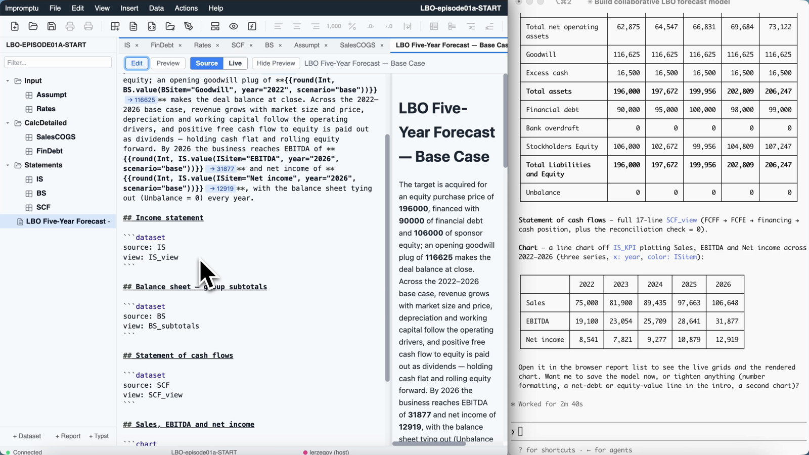
dataset: BS, view: BS_subtotals pulls the collapsed balance sheet straight out of the model, and {...} expressions interpolate live numbers into the sentences.
A report is a document stored inside the model, not an export. Its tables and charts are references to datasets and views rather than pasted copies of them. The interpolated numbers in the intro (the purchase price, the goodwill plug, 2026 EBITDA) are expressions evaluated against the live model. When an assumption changes, the prose updates with the tables, because both read the same arrays.
7. One assumption changed
The closing demonstration is the one any spreadsheet user asks for. Average sales-price growth is an assumption, 4% a year. I change it to 12% and press nothing.
Every number downstream moves. Sales rise, so receivables rise, so the capex that tracks the sales increase rises, so depreciation rises, so EBIT and net income move, so the dividend moves, so equity moves. The engine re-solves the circular system, and Unbalance again reads zero for every year.
A model that balances once is an artifact. A model that balances for every input is an instrument, and that is what makes the scenario axis, with its single base coordinate, worth having.
8. What it cost
The video is edited: Claude’s thinking and tool calls are fast-forwarded, so the video’s runtime is not the session’s. The session’s figures below are from the assistant’s own usage panel.
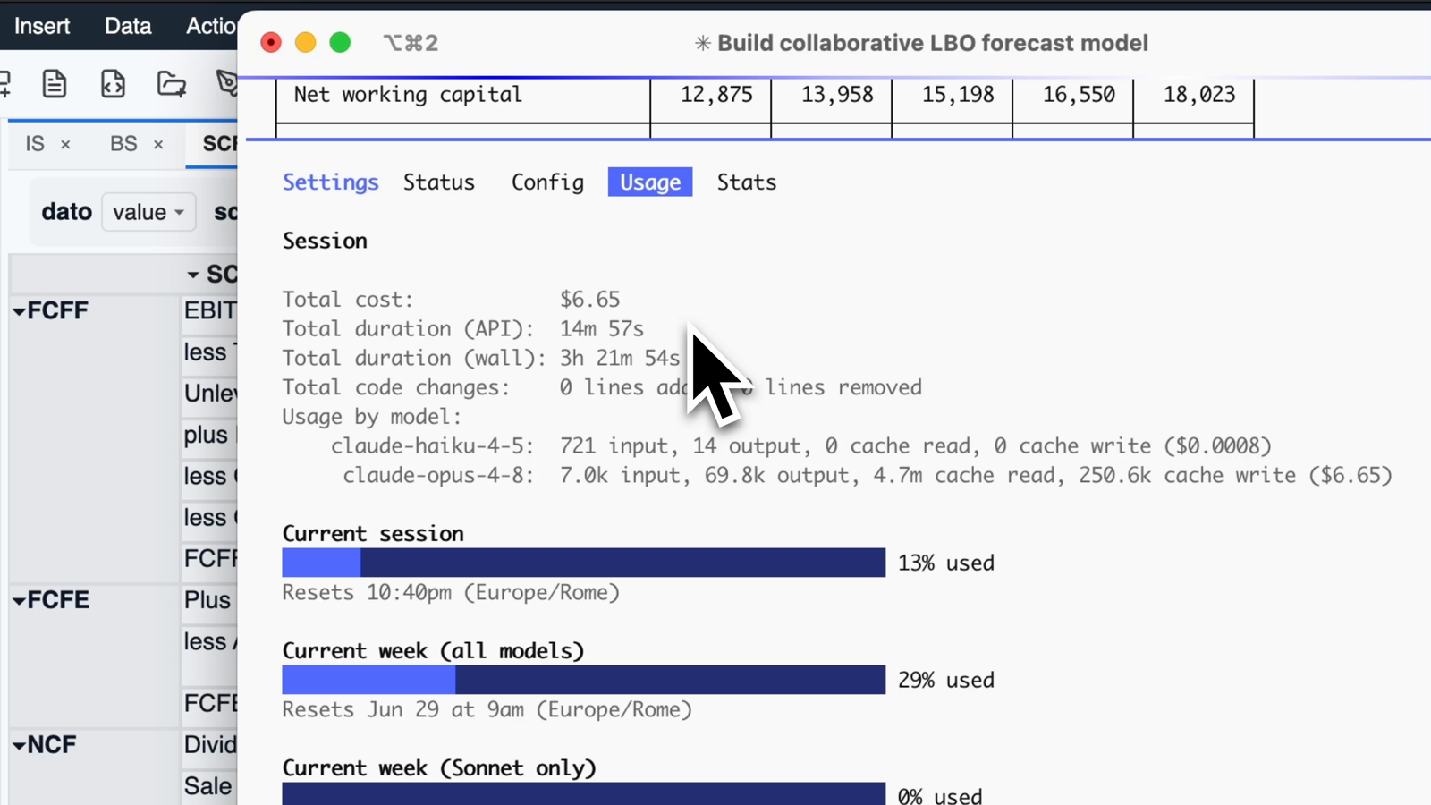
- Total cost: $6.65.
- Wall-clock: 3 hours 21 minutes 54 seconds. A working afternoon, most of it me thinking, re-recording takes and deciding what to ask next.
- API time: 14 minutes 57 seconds. That is the time the model actually spent working.
- Tokens: roughly 5.0 million, of which 4.7 million were cache reads, the model re-reading a conversation and a model structure it had already been shown. Only 69.8 thousand tokens were output: the formulas, the checks and the explanations.
- Lines of code written: zero. Nothing about the engine was touched. Everything Claude did, it did through the model’s own interface.
Six dollars and fifteen minutes of machine time built a three-statement forecast that balances. It is cheap, but that is not the reason to report it: an AI assistant in a financial workflow has a price and a duration, and both belong in the write-up next to the results. The ratio between the wall-clock and the API time describes the work: the assistant is fast, and the human deciding what to ask is the slow part.
Where this goes next
We have the flows and not yet a value. Episode 2 turns this forecast into a company valuation: a continuation value, then the adjusted-present-value and weighted-average-cost-of-capital routes to an enterprise value consistent with the financing structure, the flow-to-equity check that FCFE makes available, and the sponsor’s equity IRR.
New episodes go up on the YouTube channel. Everything permanent lives here.
Appendix A, the formulas in full
The complete formula set of the finished model, dataset by dataset, in the engine’s calculation order. Rates holds only inputs and appears nowhere below. Anything not listed here is a typed input, not a formula.
To read the listings: a bare name is a coordinate of this dataset. Dataset.name reaches into another dataset. [year:first], [year:rest] and [year:prev] are the positional operators of the recursive year dimension: the first period, all periods after the first, and the previous period. A formula with no positional qualifier applies to every year.
Assumpt, derived unit economics
The assumptions are inputs; these four lines derive the unit economics from the 2022 actuals.
market share            = company sales 000units / market size 000units
avg sales price         = Sales t0 / company sales 000units
raw material unit cost  = -Raw Materials t0 / company sales 000units
direct labor unit cost  = -Direct Labor Costs t0 / company sales 000units
SalesCOGS, the driver-led sales forecast
market size 000units[year:first]   = Assumpt.market size 000units
market size 000units[year:rest]    = market size 000units[year:prev] * (1 + Assumpt.market size g)
market share[year:first]           = Assumpt.market share
market share[year:rest]            = market share[year:prev] * (1 + Assumpt.market share g)
company sales 000units             = market size 000units * market share
avg sales price[year:first]        = Assumpt.avg sales price
avg sales price[year:rest]         = avg sales price[year:prev] * (1 + Assumpt.avg sales price g)
raw material unit cost[year:first] = Assumpt.raw material unit cost
raw material unit cost[year:rest]  = raw material unit cost[year:prev] * (1 + Assumpt.raw material unit cost g)
direct labor unit cost[year:first] = Assumpt.direct labor unit cost
direct labor unit cost[year:rest]  = direct labor unit cost[year:prev] * (1 + Assumpt.direct labor unit cost g)
FinDebt, the debt schedule
Outstanding debt is typed in by hand. One formula:
Interest = Outstanding debt[year:prev] * Rates.cost of debtBS, the balance sheet
Two arrays over the same axes: value (the balances) and delta (the year-on-year change). The last line defines the whole delta layer at once.
accounts receivable       = (Assumpt.AR days * IS.Sales) / 365
raw materials             = (-(Assumpt.raw materials days) * IS.Raw Materials) / 365
finished goods            = (-(Assumpt.finished goods days) * (IS.Raw Materials + IS.Direct Labor Costs)) / 365
wages payable             = (Assumpt.wages payable days * (IS.Direct Labor Costs + IS.Administrative)) / 365
other accounts payable    = (Assumpt.other AP days * (IS.Raw Materials + IS.Sales and Marketing)) / 365
Net working capital       = sum_group(NWC)

Net fixed assets[year:first]    = Assumpt.initial net fixed assets
Capital expenditures[year:rest] = Assumpt.capex pct of sales change * (IS.Sales - IS.Sales[year:prev])
Depreciation[year:rest]         = -(Assumpt.avg depreciation on NFA) * (Net fixed assets[year:prev] + Capital expenditures)
Net fixed assets[year:rest]     = Net fixed assets[year:prev] + Capital expenditures + Depreciation
Total net operating assets      = Net working capital + Net fixed assets

Excess cash    = SCF.Excess cash
Bank overdraft = - SCF.less Bank overdraft
Goodwill[year:first] = (Financial debt + Bank overdraft + Stockholders Equity) - (Total net operating assets + Excess cash)
Goodwill[year:rest]  = Goodwill[year:prev]
Total assets         = Total net operating assets + Goodwill + Excess cash

Financial debt = FinDebt.Outstanding debt
Net Income     = IS.Net income
Dividends      = SCF.Dividends
Sale or Purchase of Stock[year:first] = Assumpt.equity purchase price - Financial debt
Sale or Purchase of Stock[year:rest]  = SCF.Sale or Purchase of Stock
Stockholders Equity[year:first]       = Sale or Purchase of Stock
Stockholders Equity[year:rest]        = Stockholders Equity[year:prev] + Net Income + Dividends + Sale or Purchase of Stock
Total Liabilities and Equity          = Financial debt + Bank overdraft + Stockholders Equity

Unbalance = Total assets - Total Liabilities and Equity

delta = value - value[year:prev]
SCF, the statement of cash flows
The indirect method. Everything is [year:rest]: there is no cash-flow statement for the opening year, only a cash position.
EBIT[year:rest]                          = IS.EBIT
less Taxes on EBIT[year:rest]            = -EBIT * Rates.tax rate
Unlevered Net Income[year:rest]          = EBIT + less Taxes on EBIT
plus Depreciation[year:rest]             = -(IS.Depreciation)
less Changes in NWC[year:rest]           = -(BS.delta[Net working capital])
less Capex[year:rest]                    = -(BS.Capital expenditures)
FCFF[year:rest]                          = Unlevered Net Income + plus Depreciation + less Changes in NWC + less Capex

Plus net borrowing[year:rest]            = BS.delta[Financial debt]
less After tax Findebt interest[year:rest] = -(FinDebt.Interest) * (1 - Rates.tax rate)
FCFE[year:rest]                          = FCFF + Plus net borrowing + less After tax Findebt interest

Dividends[year:rest]                     = ifelse(FCFE>0,-FCFE,0)
Sale or Purchase of Stock[year:rest]     = ifelse(FCFE<0,-FCFE,0)
NCF[year:rest]                           = FCFE + Dividends + Sale or Purchase of Stock

Net cash[year:first]   = Assumpt.initial total cash
Net cash[year:rest]    = Net cash[year:prev] + NCF
Excess cash            = ifelse(Net cash>0, Net cash, 0)
less Bank overdraft    = ifelse(Net cash<0, Net cash, 0)

NCF via Income and BS delta = (IS.Net income - (BS.delta[Net working capital] + BS.delta[Net fixed assets])) + BS.delta[Financial debt] + Dividends + Sale or Purchase of Stock
The last line is a consistency check: it recomputes net cash flow from a different direction (net income less the increase in operating assets, plus net borrowing and the financing flows) and reads zero, like NCF.
IS, the income statement
Sales[year:first]                          = Assumpt.Sales t0
Sales[year:rest]                           = SalesCOGS.company sales 000units * SalesCOGS.avg sales price
Raw Materials[year:first]                  = Assumpt.Raw Materials t0
Raw Materials[year:rest]                   = -(SalesCOGS.company sales 000units) * SalesCOGS.raw material unit cost
Direct Labor Costs[year:first]             = Assumpt.Direct Labor Costs t0
Direct Labor Costs[year:rest]              = -(SalesCOGS.company sales 000units) * SalesCOGS.direct labor unit cost
Gross Profit                               = Sales + Raw Materials + Direct Labor Costs
Sales and Marketing[year:first]            = Assumpt.Sales and Marketing t0
Sales and Marketing[year:rest]             = -Sales * Assumpt.sales mktg expense on sales
Administrative[year:first]                 = Assumpt.Administrative t0
Administrative[year:rest]                  = -Sales * Assumpt.admin expense on sales
EBITDA                                     = Gross Profit + Sales and Marketing + Administrative
Depreciation[year:first]                   = Assumpt.Depreciation t0
Depreciation[year:rest]                    = BS.Depreciation
EBIT                                       = EBITDA + Depreciation
Interest on financial debt[year:first]     = Assumpt.Interest expenses t0
Interest on financial debt[year:rest]      = -FinDebt.Interest
Pre tax income                             = EBIT + Interest on financial debt
Income taxes                               = -Pre tax income * Rates.tax rate
Net income                                 = Pre tax income + Income taxes
Appendix B, Glossary
Impromptu and software
Dataset
A named matrix: a small array with named axes rather than a sheet of A1/B2 cells. A model is a handful of datasets that read each other.
Dimension and coordinate
Every axis of a dataset is a dimension; the labels along it are coordinates. The income statement’s dimensions are ISitem (its line items), year and scenario; Gross Profit is a coordinate, and 2024 is a coordinate.
Coord-formula dimension (cfd)
A dimension whose coordinates each carry their own formula. Because the line items of a statement are coordinates, there is one formula per line, written by name (Gross Profit = Sales + Raw Materials + Direct Labor Costs), and it applies across every year and scenario at once. This is the Lotus Improv idea, and it is why the formulas in this post read like accounting rather than like cell arithmetic.
Recursive dimension
A dimension, usually time, marked as ordered so that formulas can look along it. Marking year as recursive provides the positional operators [year:first] (the opening period), [year:prev] (the previous period) and [year:rest] (every period after the first), the vocabulary of a roll-forward.
Cross-dataset reference
A reference by name into another dataset: Rates.cost of debt, IS.Sales, BS.delta[Net working capital]. The bracket form selects one coordinate from a specific value layer. The model is a graph of small matrices rather than one giant sheet, and these references are its edges.
Array (value layer)
A dataset can hold several typed value layers over the same axes. The balance sheet carries two: value, the balances, and delta, the year-on-year change. delta = value - value[year:prev] is one formula that defines an entire layer.
DimGroups and sum_group
Coordinates fold into a collapsible hierarchy: Assets contains NWC contains accounts receivable. sum_group(NWC) aggregates a group by name, so the subtotal stays correct when a line is added to the group, and collapsing the group in the grid shows one row.
Pivot trays
The strips above the grid that hold each dimension. Drag a dimension between the row tray, the column tray and the page tray and the same numbers are re-arranged. No formula is retyped, because formulas were never written against a layout.
Cycle group
A set of datasets that depend on each other in a circle. The engine finds them, then iterates the group to a fixed point: here, at most 100 passes, stopping when no value moves by more than 10^{-10} in relative terms. IS, BS and SCF are one cycle group.
MCP (Model Context Protocol)
A standard by which an AI assistant’s host application connects to external tools and data. Here it is the bridge that lets Claude list datasets, read and write formulas, recalculate and read results back, operating the live model rather than describing one.
Finance
LBO (leveraged buyout)
The purchase of a company financed largely with borrowed money, where the acquired company’s own cash flows service the debt. Here: 196,000 of purchase price, 90,000 of it debt.
Working-capital days
A driver that expresses a balance as a number of days of the flow that produces it. accounts receivable = AR days × Sales / 365 says customers pay in 60 days. Inventories are expressed in days of the costs that build them; payables in days of the costs they finance.
Indirect cash-flow method
Deriving cash flow from accrual accounts rather than from a cash ledger: start from earnings net of taxes, subtract changes in net assets and add changes in net liabilities. It is the method that lets a cash-flow statement fall out of an income statement and a balance sheet. It can be applied as if the firm had no debt to get FCFF, or including debt to get FCFE.
FCFF and FCFE
Free cash flow to the firm is the cash the operations generate for all providers of capital, computed as if the firm had no debt: after-tax EBIT + depreciation − change in net working capital − capex. Free cash flow to equity is what is left for shareholders after the debt is served: FCFF + net borrowing − after-tax interest.
The goodwill plug
When a buyer pays more than the identifiable net assets are worth, the difference is capitalized as goodwill so the opening balance sheet balances. Here 196,000 paid − 62,875 of net operating assets − 16,500 of cash = 116,625 of goodwill, carried forward unchanged.
Roll-forward
Any balance defined as opening balance + additions − subtractions = closing balance. Fixed assets roll forward with capex and depreciation; equity rolls forward with net income, dividends and stock issues. In a recursive dimension a roll-forward is one line: X[year:rest] = X[year:prev] + inflow - outflow.
Average depreciation rate on the net asset base
The rate this model applies: 10% of net fixed assets (last year’s closing balance plus this year’s capex), not the statutory rate a tax code applies to an asset’s gross cost over a fixed life. It is a planning shortcut, one rate standing in for a whole schedule of assets of different ages and lives, suited to a five-year forecast and not to a tax filing.
The unbalance check
A line whose formula is Total assets − Total Liabilities and Equity and whose only acceptable value is zero. A model without one is a model whose author has not checked.
FCFE absorption
The cash policy used in this model: every year’s free cash flow to equity is paid out as a dividend if positive, or covered by a stock issue if negative, so net cash flow is zero and cash never moves. It is a deliberate simplification that lets the circular system close without a solver. Relaxing it makes the residual reappear as excess cash or a bank overdraft, the two lines at the bottom of the balance sheet.