Valuing a company with an AI assistant
Episode 2 of the AI-assisted financial analysis series. Last time I built a company: a five-year income statement, balance sheet and cash-flow forecast for a leveraged buyout, mostly written by an AI assistant. This time I put a price on it. Three valuation methods discount the same cash flows at three different rates, and if the model is right they agree on one equity value. I do the one piece of algebra worth doing by hand and hand the rest to the assistant. This post is the canonical write-up. The video below is the short version, and everything here is readable on its own. It follows directly from Episode 1, whose company I am now valuing.
The result, and the bench in one minute
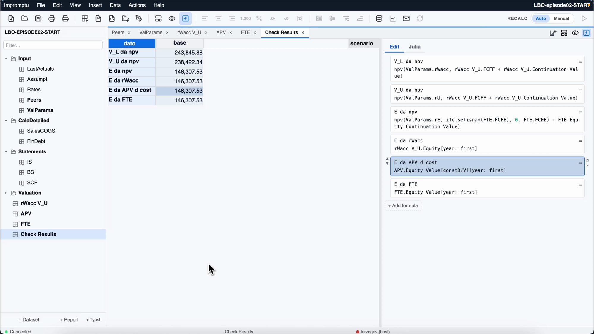
Check Results table. Equity value by the weighted-average-cost-of-capital method, by adjusted present value at constant leverage, by flow to equity and by an independent npv() restatement: all four read 146,307.53.
Three valuation methods, built on the same forecast, discount the same cash flows at three different rates, and the four figures in that table read 146,307.53 (thousands, throughout). This post builds that table, explains why those four numbers cannot disagree, and shows the one number in the model that deliberately does.
Three things are on the bench in this episode.
The Workbench is this site: field notes from an ongoing experiment in building small, transparent tools for teaching finance and for probing how AI works. The manifesto says why. The blog is the permanent home; the videos are demonstrations.
Impromptu is the modeling engine on screen. It is a multidimensional spreadsheet in the tradition of Lotus Improv, a tradition that continues in Quantrix Modeler, the tool of our Financial Planning Lab at Trento. In a multidimensional spreadsheet there is no =B7*C7 to drag down. The formula is Equity = V_L - Debt, written once over a whole named array, and it applies to every year and every scenario at once. Impromptu is a research prototype, not a product and not a replacement for the tools we teach with. It exists because some questions can only be answered with an instrument that can be taken apart. What is running is the subject of a separate note.
Claude Code is the AI assistant. It is wired to the live engine: connected through MCP (the Model Context Protocol), it can list datasets, read existing formulas, write new ones, recalculate and read the results back, while I watch every step. When the assistant writes a formula, that formula lands in the model the way mine does, in the same readable language.
Technical terms are named where they first appear and collected in the glossary. The complete formula set is in Appendix A, so a reader can rebuild the valuation in the tool of their choice.
What made it valuation-ready
The forecast is where Episode 1 left it: income statement, balance sheet and cash flow, all balancing, for a manufacturer bought at the end of 2022 for 196,000, with 90,000 of bank debt. Two small changes carried over from that build matter for the valuation.
The first is a tidying. The company’s 2022 actuals (last year’s sales, costs and the opening asset base) now live in their own dataset, LastActuals, which has no scenario axis. History does not change in a what-if, so it should not sit on the same axis as the assumptions that do. Assumpt now holds only the drivers that vary by scenario. That separation is what lets the scenario axis, later in the post, do its work without touching the past.
The second is a policy, and it is what makes the valuation possible. In Episode 1 the cash line was flat on purpose: every year’s free cash flow to equity is paid out as a dividend if positive, or covered by a stock issue if negative, so net cash flow is zero and the cash balance never moves. That is the FCFE policy (free cash flow to equity). No cash piles up on the balance sheet and no financing plug moves, so the value of the business rests on its free cash flows and nothing else. A model that hoards cash forces an argument about what the cash is worth. This one does not.
The one piece of algebra, the cost of capital
Discounting needs a cost of capital, and the cost of capital needs the company’s own risk, its beta. This company is private and does not trade, so its risk is borrowed from firms that do.
I take two listed peers, Tusk and Sangyo, and strip their financing out. The unlevered (asset) beta is the value-weighted average of a firm’s equity and debt betas: the business risk the firm would carry with no debt. This is the one formula I write by hand, on camera, in the model’s own language:
betaU[peer:butlast]     = betaE*(1-D/V) + betaD*D/V
betaU[industry average] = mean(betaU[peer:butlast], dims=Dim{:peer})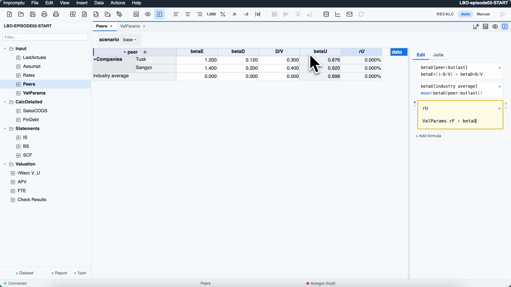
Peers dataset. Two companies, with their equity betas, debt betas and leverage typed in, and the asset beta betaU computed by the unlevering formula in the editor pane on the right. Tusk unlevers to 0.876, Sangyo to 0.920, and the industry average row, a slice of the two companies only, averages them to 0.898.
Two details in that formula matter. [peer:butlast] means every peer except the last: the two real companies, without the industry average summary row beneath them. The average is taken over that same slice, mean(betaU[peer:butlast], …), so the summary row is the mean of the companies and does not include itself. (This is the sliced-mean fix that gives this build its betafixed name; an earlier version averaged over the whole column, including the blank summary cell.)
The two peers differ in equity beta, 1.20 against 1.40, and barely in asset beta, 0.876 against 0.920. Most of the gap was leverage rather than business risk. That convergence is the justification for the exercise: with the financing stripped out, the two firms look like two companies in the same line of work. I take their average, βU = 0.898, as the company’s asset risk.
From there, one line of CAPM prices any beta: r = r_F + \beta \cdot \text{MRP}, a risk-free rate plus beta times the market risk premium. With r_F = 4\% and a premium of 5.5\%, the asset beta gives the unlevered cost of capital:
r_U = r_F + \beta_U \cdot \text{MRP} = 4\% + 0.898 \times 5.5\% = 8.94\%
That is the rate the business earns before any financing decision, and the anchor for everything that follows.
Then the leverage goes back in. Modigliani–Miller Proposition II says that leverage does not create value but redistributes risk: equity holders bear the business risk plus a premium for the debt ranking ahead of them. Relevering at a target debt ratio of D/V = 40\% (so D/E = 0.667), with a debt cost r_D = 4.44\%:
r_E = r_U + (r_U - r_D)\cdot\frac{D}{E} = 8.94\% + (8.94\% - 4.44\%)\times 0.667 = 11.94\%
Finally the blend, the weighted average cost of capital, the after-tax average of what the two claims cost:
r_{WACC} = r_E\cdot\frac{E}{V} + r_D(1-T)\cdot\frac{D}{V} = 8.32\%
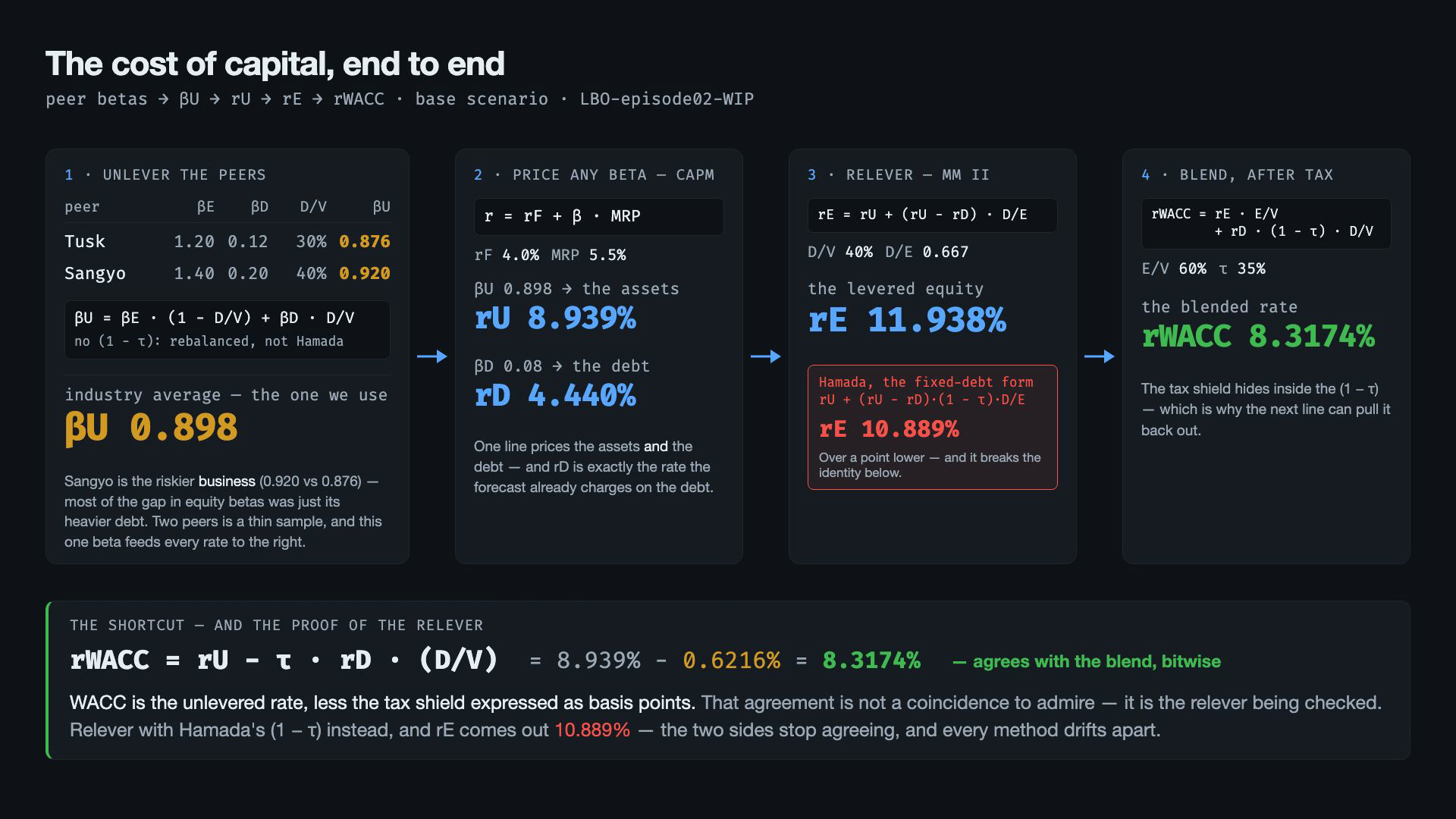
The WACC, 8.32 %, is below rU’s 8.94 %. The gap of roughly 0.62 % is the tax shield, the subsidy the tax code gives a levered firm because interest is deductible. The model carries the WACC a second way, as the shortcut r_U - r_D \cdot (D/V) \cdot T, and the two agree to eleven decimal places. The agreement is an algebraic identity, and it is the assistant’s proof that it relevered correctly. Read that way, r_{WACC} is the unlevered rate with the tax shield subtracted, and every method below follows from that.
The assistant wrote everything on that map from rD down to rWacc: I described the cost of capital in plain finance and it produced the formulas. As soon as the peer betas existed, the ValParams dataset that depends on them recomputed, the way a spreadsheet recomputes, except that here the cell is a whole named quantity and the formula reads like the textbook line it implements.
Three roads to one value
With a cost of capital in hand, the company can be valued three ways.
Road one, the WACC benchmark
Discount the free cash flow to the firm at the WACC. The mechanics show what the year dimension is for. No forecast runs forever, so at the horizon the model takes a continuation value: the last year’s EBITDA times an EV/EBITDA multiple of 6.8, a simple and defensible anchor for everything after 2026. The discounting is then a backward recursion rather than one long sum: each year’s value is next year’s cash flow plus next year’s value, discounted one period. It is written once, with a [year:next] reference, and the engine rolls it back from the horizon to today:
V_L[year: last]    = Continuation Value
V_L[year: butlast] = (FCFF[year: next] + V_L[year: next]) / (1 + rWacc)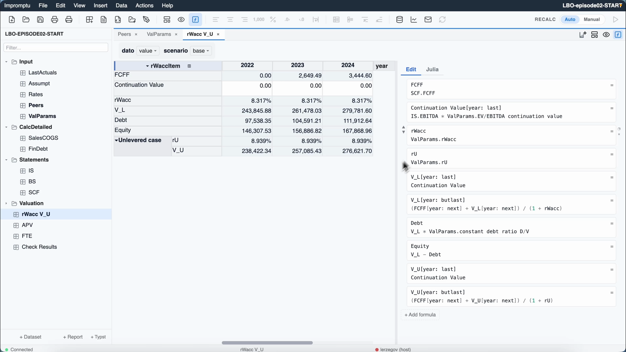
rWacc V_U dataset. The backward recursion in the editor (V_L[year: butlast] = (FCFF[year: next] + V_L[year: next]) / (1 + rWacc)), and the results in the grid. Levered value V_L = 243,845.88, the zero-debt baseline V_U = 238,422.34, and equity 146,307.53.
The same dataset runs the recursion a second time at the unlevered rate rU, giving V_U = 238,422.34, what the same cash flows would be worth to a firm with no debt. That is the baseline the next method builds on. The levered value is 243,845.88; 40 % of it is debt, and subtracting the debt leaves equity of 146,307.53.
Road two, the APV bridge and the debt-policy lesson
The adjusted present value method values the pieces separately: take the business as if it were unlevered, then add the value of the tax shield the debt creates.
V_L = V_U + PV(\text{tax shields})
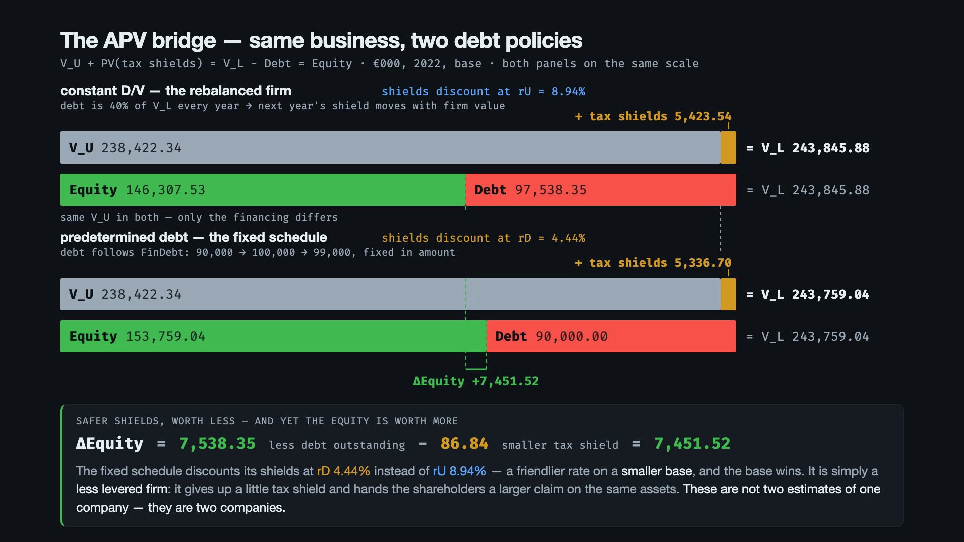
The virtue of APV is that the tax shield becomes a visible line item with its own cash flows and its own discount rate, and that discount rate is where debt policy enters. The model carries one dataset with two debt policies side by side, and the assistant writes only the two formulas that differ between them; every other line is written once and shared:
- Constant debt ratio. Debt is rebalanced to 40 % of firm value every year, so future debt rises and falls with the business. The shields are as risky as the assets and are discounted at rU. This branch reads equity 146,307.53, the same as the WACC benchmark.
- Predetermined schedule. Debt follows the LBO’s amortisation plan (90,000 → 100,000 → 99,000), fixed in advance. The shields are about as safe as the debt itself and are discounted at the lower rD. This branch reads equity 153,759.04.
Same company, same cash flows, seven million euros of difference (millions, because the model’s figures are in thousands). The answer moved with the financing assumption and not with the method. That is the lesson of the episode, and the reason the model keeps both policies in view.
Road three, flow to equity
The third road skips the firm and values the shareholder’s claim directly. Build the cash flow to equity (free cash flow to the firm, less the after-tax interest paid to lenders, plus any net new borrowing) and discount it at the cost of equity, 11.94 %:
FCFE       = FCFF + less after tax Interest + change in Debt
Equity Value[year: butlast] = (FCFE[year: next] + Equity Value[year: next]) / (1 + rE)
It is the most laborious of the three, since it needs the full debt schedule and the levered rate, and for the same reason it is the best cross-check: if the debt in the cash flow and the leverage in the rate disagreed, this is where it would show. It reads 146,307.53.
Proving it, the reconciliation
A printed agreement is worth less than a proved one. So the last valuation step re-values everything a second way, with plain npv() net-present-value formulas of the kind any spreadsheet has, and asks which numbers must coincide, and why. That is the Check Results table at the top of this post: the levered value by npv matches the recursion, and equity by WACC, by APV (constant ratio), by flow to equity and by the independent npv restatement all read 146,307.53.
The agreement is an identity. The three methods are one proposition written three ways: the same cash flows, the same debt policy, three arrangements of the same algebra. The full proof (why WACC is APV under the constant-ratio assumption, and why the flow-to-equity recursion telescopes into V_L - D) is in the teaching note, because it is the assistant’s own to make.
One number in the model does not join in: the predetermined-schedule equity, at 153,759. It is the control, a different financing assumption giving a different answer. If that one had matched, I would know something was broken. A reconciliation is convincing only if the thing that should not reconcile is also shown, and does not.
The analyst’s note
Up to this point the assistant has worked inside my datasets, my structure and my pipeline. In the last step I ask it to do what a certified analyst does and explain the model: not only the numbers but the theory, the propositions, the debt-policy debate and when a practitioner should reach for each method, with every word grounded in this model’s own figures.
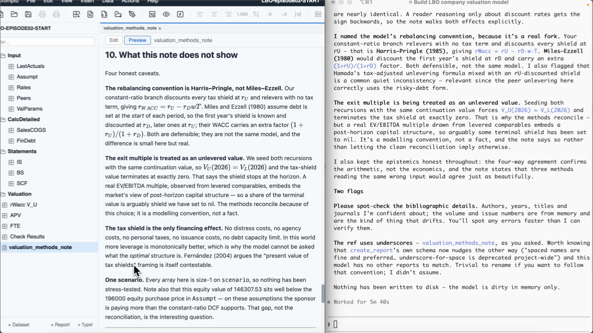
What comes back is a teaching note: the peer analysis, the cost-of-capital chain, all three methods with the model’s tables, the reconciliation above, and the classic papers named where they bear on what is on screen. It is long and it is its own document, so it lives on a companion page:
→ Read the full teaching note the assistant generated: DCF valuation under alternative debt policies.
One thing it flags belongs here, because it is the difference between a tool and an analyst. The continuation value uses an EV/EBITDA multiple of 6.8, seeded identically into the levered and unlevered recursions. The note points out that this implies a long-run growth rate of around 6 %, and that seeding both recursions the same way sets the terminal tax shield to exactly zero, a modelling convention rather than a fact, and one the reconciliation depends on. It also states the limit of the check: the four-way agreement, it says, “confirms the arithmetic, not the economics — three methods reading the same wrong input would agree just as beautifully.” That is judgement.
The scenario axis, best and worst case
One more step shows what the structure was for. The model was built scenario-ready from the start: every valuation dataset carries a scenario axis that, until now, held only base. I add a best case and a worst case, as input numbers only: growth rates, margins, betas.
The claim is that this takes no new formulas: the structure is described once and every what-if follows. It very nearly holds. Every valuation dataset recomputes for all three scenarios at once, but adding the scenarios surfaced two things the assistant had to fix, and the video shows it catch and repair each one, live.
The first was an average with no axis named. The industry asset beta is the mean of the two peers, betaU[industry average] = mean(betaU[peer:butlast]). With one scenario that bare mean() returned the right number; with three, it collapsed the scenario axis as well as the peer axis and averaged the three cases into a single beta. The size of the axis had been standing in for its name: length one hides the mistake and length three exposes it. The fix pins the reduction to the peer axis, mean(betaU[peer:butlast], dims=Dim{:peer}), averaging the peers within each scenario. (That correction is why the model behind this post is the one named betafixed.)
The second was subtler, and it is a lesson about what follows from the structure and what does not. A formula fans out across a new scenario automatically; that is the point of the axis. A typed input does not: it is a value, not a rule, so it has to exist for every scenario or it is blank. Most scenario inputs get entered, because they are what the scenario is about: the growth rates, the margins, the betas. The one that gets forgotten is the debt schedule, the LBO’s contractual repayment plan, 90,000 rising to 100,000 and amortising to 99,000, which I typed in back in Episode 1 and which is the same in every scenario because it is a signed loan agreement, not a forecast. When the best and worst columns appeared, that schedule was blank in them, and empty debt would have broken the interest line and the predetermined-debt valuation. The assistant caught the gap and copied the base schedule across, which is right: growth rates and margins change from case to case and the debt does not.
This was not the first time the scenario axis found a defect. An earlier session, not the one recorded here, had used it to find a worse one. References that reach across datasets were being matched by axis position rather than by name, and the forecast and valuation datasets order their scenario axis at opposite ends. With a single scenario every axis is length one and lines up by chance; with three, figures from one scenario landed under another and base equity came out at roughly half the true value, while the balance sheet still tied to zero, the three methods still agreed with each other, and every npv() check still reconciled. A bug that keeps every check green while the answer is wrong by half is the most dangerous kind. It took a dedicated engineering session to trace and repair, in the engine rather than in a formula. A new axis is the instrument that finds such things.
With both fixed, base equity holds at 146,307.53, the best case reads 235,270 and the worst 63,174, and the three methods agree in every scenario.
What it cost
The video is edited: the assistant’s thinking and tool calls are fast-forwarded, so the video’s runtime is not the session’s. The session’s real figures follow. I report them because an AI assistant in a financial workflow has a price and a duration, and both belong next to the results.
- API time: 25 minutes 24 seconds, the time the model spent working.
- Tokens: roughly 15.2 million, of which about 14.7 million were cache reads: the model re-reading a conversation and a model structure it had already been shown, turn after turn. The new output (the formulas, the checks, the teaching note) is a thin slice on top of that.
- Cost: $13.57 (Opus 4.8, with a few cents of Haiku).
Thirteen dollars and twenty-five minutes of machine time valued a company three ways, proved the three agree, and wrote the analyst’s note, on a forecast that itself cost six dollars in Episode 1. The cache-read figure is the shape of the work: most of the cost is the assistant holding the whole model in view while it reasons about one more line.
Where this goes next
The company has a value, shown to be the same by three methods, and the disagreements that matter come from the assumptions rather than from the choice of formula. Next in the series: a cost of capital that changes year to year, and real cash on the balance sheet, excess cash and overdrafts instead of the flat-cash policy that kept this one simple.
New episodes go up on the YouTube channel. Everything permanent lives here.
Appendix A, the formulas in full
The complete formula set, dataset by dataset, pulled live from the finished betafixed model in the engine’s calculation order. Anything not listed is a typed input, not a formula.
To read the listings: a bare name is a coordinate of the current dataset. Dataset.name reaches into another dataset. [year:first], [year:last], [year:prev] and [year:next] are positional operators of the recursive year dimension (the first period, the last, the one before, the one after), and [year:butlast] means every year except the last. [peer:butlast] is the same idea on the peer axis. A formula with no positional qualifier applies across every coordinate at once.
LastActuals, the 2022 unit economics
Scenario-free. These four lines derive the unit economics from the 2022 actuals; the forecast engine reads them for its opening year.
market share           = company sales 000units / market size 000units
avg sales price        = Sales t0 / company sales 000units
raw material unit cost  = -Raw Materials t0 / company sales 000units
direct labor unit cost  = -Direct Labor Costs t0 / company sales 000units
Peers, the unlevered beta
betaU[peer:butlast]     = betaE*(1-D/V) + betaD*D/V
betaU[industry average] = mean(betaU[peer:butlast], dims=Dim{:peer})
rU                      = ValParams.rF + betaU * ValParams.CAPM market risk premium
The first line is the sliced-β formula: it computes an asset beta for the two real companies ([peer:butlast]) and leaves the industry average row to the second line, which averages only those companies.
ValParams, the cost of capital
betaU             = Peers.betaU[industry average]
constant tax rate = Rates.tax rate
rU     = rF + betaU*CAPM market risk premium
rD     = rF + betaD*CAPM market risk premium
D/E    = (constant debt ratio D/V)/(1-(constant debt ratio D/V))
rE     = rU + (rU-rD)*(D/E)
rWacc  = rE*(1-(constant debt ratio D/V)) + rD*(1-constant tax rate)*(constant debt ratio D/V)
rWacc shortcut = rU - rD*(constant debt ratio D/V)*constant tax rate
The last two lines are the WACC computed two ways, the definitional blend and the shortcut r_U - r_D(D/V)T.
Rates, the debt cost
One formula. In this model the cost of debt is deliberately tied to the CAPM debt cost rD, so that the constant-ratio APV and the WACC method reconcile exactly rather than approximately.
cost of debt = ValParams.rDrWacc V_U, the WACC benchmark and the zero-debt value
FCFF               = SCF.FCFF
Continuation Value[year: last] = IS.EBITDA * ValParams.EV/EBITDA continuation value
rWacc              = ValParams.rWacc
rU                 = ValParams.rU
V_L[year: last]    = Continuation Value
V_L[year: butlast] = (FCFF[year: next] + V_L[year: next]) / (1 + rWacc)
Debt               = V_L * ValParams.constant debt ratio D/V
Equity             = V_L - Debt
V_U[year: last]    = Continuation Value
V_U[year: butlast] = (FCFF[year: next] + V_U[year: next]) / (1 + rU)
APV, adjusted present value with two debt policies
The apvModel dimension carries two policies, predetD and constD/V. Only Debt and the shield’s discount rate rT differ between them; every other line is written once and shared.
Debt[predetD]  = FinDebt.Outstanding debt
Debt[constD/V] = rWacc V_U.Debt
rT[predetD]    = ValParams.rD
rT[constD/V]   = ValParams.rU
Interest       = Debt[year: prev] * Rates.cost of debt
Tax Shield     = Interest * ValParams.constant tax rate
Tax Shield Value[year: last]    = 0
Tax Shield Value[year: butlast] = (Tax Shield[year: next] + Tax Shield Value[year: next]) / (1 + rT)
V_U            = rWacc V_U.V_U
V_L            = V_U + Tax Shield Value
Equity Value   = V_L - Debt
FTE, flow to equity
FCFF                    = rWacc V_U.FCFF
less after tax Interest = -(APV.Interest[constD/V]) * (1 - ValParams.constant tax rate)
change in Debt          = APV.Debt[constD/V] - APV.Debt[constD/V][year: prev]
FCFE                    = FCFF + less after tax Interest + change in Debt
rE                      = ValParams.rE
Equity Continuation Value[year: last] = rWacc V_U.Continuation Value - rWacc V_U.Debt
Equity Value[year: last]    = Equity Continuation Value
Equity Value[year: butlast] = (FCFE[year: next] + Equity Value[year: next]) / (1 + rE)
Check Results, the reconciliation
V_L da npv       = npv(ValParams.rWacc, rWacc V_U.FCFF + rWacc V_U.Continuation Value)
V_U da npv       = npv(ValParams.rU, rWacc V_U.FCFF + rWacc V_U.Continuation Value)
E da npv         = npv(ValParams.rE, ifelse(isnan(FTE.FCFE), 0, FTE.FCFE) + FTE.Equity Continuation Value)
E da rWacc       = rWacc V_U.Equity[year: first]
E da APV d cost  = APV.Equity Value[constD/V][year: first]
E da FTE         = FTE.Equity Value[year: first]
The forecast engine, carried from Episode 1
The datasets that produce the cash flows (SalesCOGS, FinDebt, IS, BS, SCF) are the ones built in Episode 1, essentially unchanged except that their opening-year inputs now read from LastActuals rather than from Assumpt. Their full formulas are in that post’s Appendix A. The only line the valuation reads directly is SCF.FCFF, the free cash flow to the firm, which feeds rWacc V_U above.
Appendix B, Glossary
Two short glossaries. Terms shared with Episode 1 (dataset, dimension and coordinate, coord-formula dimension, recursive dimension, cross-dataset reference, sum_group, cycle group, MCP, LBO, FCFF/FCFE) are defined in the Episode 1 glossary; this one adds what is new in Episode 2.
Impromptu and software
Positional slices, [year:next] and [peer:butlast]
The recursive dimensions provide a vocabulary for looking along an axis. Beyond Episode 1’s first/prev/rest, this model uses [year:next] (the following period, which is how the backward recursion reads next year’s value), [year:last] and [year:butlast] (the horizon, and every year before it), and the same idea on the peer axis: [peer:butlast] selects every peer except the summary row. A slice is how one formula selects some coordinates and not others without leaving the named world for cell arithmetic.
The apvModel per-model dimension
An axis whose coordinates are whole modelling assumptions rather than time or line items: here, the two debt policies predetD and constD/V. A formula written once applies to both; a formula written [predetD] or [constD/V] applies to one. It is how a single dataset holds a controlled comparison: everything shared is written once, and only the two lines that differ are split. The model makes the claim structurally: these are not two methods, they are one method under two assumptions.
npv()
The ordinary net-present-value function every spreadsheet has: npv(rate, cashflows) discounts a stream at a flat rate. The model uses it in Check Results as an independent restatement of values it computed by backward recursion, a deliberately different piece of machinery, so that agreement between them is a check and not a tautology.
Finance
Beta, and unlevered (asset) beta
Beta measures how much an asset’s return moves with the market. A listed firm’s equity beta (\beta_E) includes the effect of its leverage; with the financing stripped out it becomes the unlevered (asset) beta (\beta_U), the risk of the underlying business. Unlevering is \beta_U = \beta_E(E/V) + \beta_D(D/V): the asset is a portfolio of the claims on it, so its beta is their value-weighted average.
rU, rE, rWacc
Three costs of capital for the same firm. rU (8.94 %) is the return demanded on the assets, before any financing. rE (11.94 %) is what equity holders demand once debt ranks ahead of them. rWacc (8.32 %) is the after-tax weighted average of what debt and equity cost. Because interest is tax-deductible, it sits below rU by exactly the tax shield.
Modigliani–Miller and relevering
The Modigliani–Miller propositions say that, in a frictionless world, capital structure does not create value (Proposition I); it only redistributes risk, so the cost of equity rises with leverage (Proposition II): r_E = r_U + (r_U - r_D)(D/E). Relevering uses that identity to convert an asset return back into an equity return at a chosen debt ratio.
WACC-DCF, continuation value and the exit multiple
The WACC discounted-cash-flow method values a firm by discounting its free cash flow to the firm at the WACC. No forecast runs forever, so the horizon is capped with a continuation (terminal) value, here an exit multiple: the last forecast year’s EBITDA times an assumed EV/EBITDA ratio (6.8). It is the simplest defensible anchor for everything beyond the forecast.
V_U and V_L
The unlevered and levered enterprise values. V_U (238,422) is what the business is worth financed entirely by equity; V_L (243,846) is what it is worth with the debt in place. The difference is the value of the tax shield.
Tax shield
The value created purely because interest is tax-deductible: the tax authority effectively pays a fraction of the interest bill. It is the gap between V_L and V_U, the gap between rU and rWacc, and, in APV, an explicit line item with its own cash flows.
APV (adjusted present value)
Valuing the levered firm in pieces: V_L = V_U + PV(\text{tax shields}). Value the business unlevered, then add the financing side-effects separately. Its virtue is transparency: the tax shield is a visible number with its own discount rate rather than a term inside a WACC, which is why it is the natural language of the leveraged buyout.
Flow to equity (FTE)
Valuing equity directly: build the cash flow that reaches shareholders (FCFF, less after-tax interest, plus net new borrowing) and discount it at the cost of equity, rE. No tax shield appears, because the interest is already deducted at its after-tax cost inside the cash flow.
Constant debt ratio vs predetermined (fixed) debt schedule
The debt-policy choice of the episode. Under a constant debt ratio the firm rebalances debt to a fixed fraction of its value every year, so future debt is unknown today and moves with the business; the tax shields carry the business risk and are discounted at rU (the Harris–Pringle convention). Under a predetermined schedule the euro amounts of debt are fixed in advance, so the shields are as safe as the debt and are discounted at rD (the Modigliani–Miller / Myers convention). Same firm, same cash flows, different equity value, because the two policies describe different companies.
The reconciliation identity
The fact that the WACC, constant-ratio APV and flow-to-equity methods must give the same equity value when their assumptions are made consistent, because r_{WACC} = r_U - r_D(D/V)T is exactly “discount at rU and add the shield back,” which is what APV does explicitly and what FTE does implicitly. Agreement confirms the arithmetic; it is a necessary check, never a sufficient one.