Paying out, paying down: cash policy and the circular model
Episode 3 of the AI-assisted financial analysis series. Episode 1 forecast a company’s statements and Episode 2 valued it. Neither decided what the company does with the cash it makes. This episode does, and the decision brings interest on a balance that depends on the interest. The video shows the edits as they happen. This post carries the derivations the video only mentions, the iteration counts with the rule used to count them, and a correction to Episode 1.
The result in brief
The company from the first two episodes gets three cash policies. One of them repays debt fast enough to run an overdraft at 8%. Interest on a balance that depends on the interest can make a model circular, and whether it does depends on when interest is credited.
- Credited once a year, at year end, there is no loop. The model computes the balance before interest, charges interest on the average balance, and adds it at the close. It is exact under that convention.
- Accrued within the year, the average balance includes this year’s interest, so the interest depends on itself. Impromptu refuses that loop inside one dataset and converges it across two.
- The two conventions differ by 4.25 on the 2026 cash balance of the cash-rich policy and by 181.18 under the overdraft policy. Neither number is an error. Each is the price of a convention, and a slightly higher equivalent rate closes the gap everywhere except in the year the balance crosses zero.
The model is built in Impromptu, my own research bench, a multidimensional spreadsheet in the tradition of Lotus Improv and Quantrix Modeler. It is described in a separate note; it is not a product and cannot be downloaded. The AI assistant is Claude Code, connected to the live engine through MCP, as in the earlier episodes. Amounts are in thousands. Technical terms are collected in the glossary and the formulas in Appendix A.
The cash nobody decided about
Episode 2’s model paid free cash flow to equity (FCFE) out as dividends when it was positive and covered it with a stock issue when it was negative. Cash stayed flat, and the valuation could rest on free cash flows alone. That was a simplification, and it left a question open: what does the company do with the cash it makes?
The starting model for this episode already separates two kinds of cash. Operating cash is the minimum the business needs to run. Discretionary cash is the rest, and it is either excess cash earning 2% or, when it goes negative, a bank overdraft costing 8%. Both rates are inputs in the Rates dataset. The cash statement SCF computes the balance year by year.
Three policies on one axis
A cash policy is a set of inputs, so three policies are three coordinates of the scenario dimension. I asked Claude to add two beside base:
| policy | dividends, share of FCFE | financial debt, 2022 to 2026 |
|---|---|---|
base |
60% | 90,000 → 95,000 → 100,000 → 98,000 → 99,000 |
payout |
100% | as base |
deleverage |
100% | 90,000 → 70,000 → 50,000 → 30,000 → 10,000 |
Everything else is the base column copied across. No formula changed. The formulas are written over whole arrays, so a new coordinate of an existing dimension is computed by the formulas that are already there. Episode 2 showed this with a best and a worst case. Here the axis is setup for the rest of the episode.
By 2026, base and payout still hold excess cash. deleverage repays 80,000 of debt in four years, and its discretionary balance crosses zero in 2023, from +10,335.62 to −10,964.32, and ends 2026 overdrawn by 73,211.13.
Interest on the balance
Overdraft interest is 8% of the average overdraft over the year. The average depends on the balance at the end of the year. The balance at the end of the year depends on how much interest was paid. Written that way, the interest depends on itself.
The starting model does not have that loop. The reason is a convention about when interest is credited, and it is written in the formulas.
Credited once a year: why SCF has no loop
SCF computes the year in two passes. The first is the cash flow before cash interest, which is what BCI means in the line names:
NCF BCI               = FCFE + Sale or Purchase of Stock + Dividends + Re-add change in operating cash
Net cash position BCI[year:rest] = Net cash position[year:prev] + NCF BCI
Discretionary BCI     = Net cash position BCI - BS.Minimum operating cash
The average balance for the year is taken between last year’s closing balance (Discretionary prev) and Discretionary BCI, the balance before this year’s interest. Interest is charged on that average, taxed, and only then added to the cash flow and to the closing balance:
Cash interest income[year:rest]       = Rates.excess cash interest rate * Avg excess cash
Overdraft interest expense[year:rest] = Rates.overdraft interest rate * Avg overdraft
After tax cash interest[year:rest]    = Net cash interest * (1 - Rates.tax rate)
NCF                                   = NCF BCI + After tax cash interest
The year’s interest joins the balance on 31 December and earns nothing until the next year. That is annual compounding. Discretionary BCI is not an estimate of the closing balance: it is the balance to which this convention applies interest. Under that convention the model is exact.
The average balance, in closed form
The two average lines in SCF are four-branch switch formulas on the signs of the opening and closing balances (the full text is in Appendix A). They compute the time-weighted average of a balance that moves in a straight line from a at the start of the year to b at the end, split into its positive part (excess cash) and its negative part (overdraft).
The four branches reduce to one expression. Write x^+ = \max(x, 0). The average of the positive part over the year is
\overline{x^+} = \frac{(a^+ + b^+)^2}{2\,(|a| + |b|)} .
In a year where a and b have the same sign, |a| + |b| = a^+ + b^+ and the expression reduces to the midpoint (a^+ + b^+)/2. In a year where the balance crosses zero, one of a^+, b^+ is zero. If the positive one is a^+, the balance is above zero for a fraction a^+/(|a|+|b|) of the year, at an average height of a^+/2. The product is the area of a triangle, which is the expression above. The overdraft average is the same expression on a^- and b^-.
I checked both forms against a numerical quadrature of the true time average over 33 sign cases. The switch and the closed form agreed with a maximum difference of 0.0, and both were within 5e-8 of the quadrature, which is the quadrature’s own error.
Subtracting the two averages removes the crossing:
\overline{x^+} - \overline{x^-} = \frac{a + b}{2} .
The net average balance is always the midpoint. The zero crossing only decides how that midpoint is split between the 2% deposit rate and the 8% overdraft rate. Under deleverage in 2023, the year the balance crosses zero (from +10,335.62 to −10,966.76 in SCF recursive, the within-year statement of the sections below), the averages are 2,507.35 of excess cash and 2,822.92 of overdraft, and their difference is the midpoint, −315.57.
The refusal: a loop inside one dataset
Suppose interest accrues during the year instead. Then the average should read the balance including this year’s interest. In SCF that is one edit: delete BCI from
Discretionary BCI = Net cash position BCI - BS.Minimum operating cashso that the line reads Net cash position, the balance after interest. Impromptu refuses the edit:
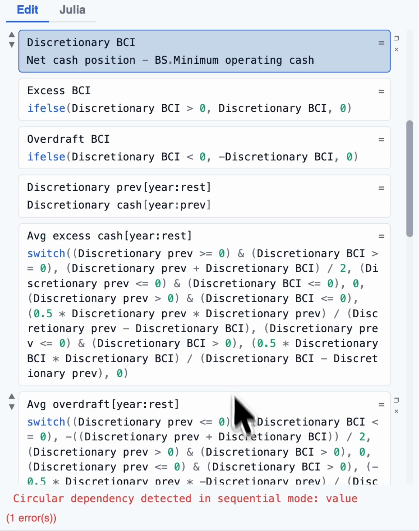
Discretionary BCI, now reading Net cash position. The red line at the foot is the engine’s answer, and the model keeps its previous formulas.
Circular dependency detected in sequential mode: value. The model keeps its old formulas and its old values. The same message comes back for three other circular edits I tried, including moving the interest multiplications of the next section back inside one dataset.
The reason is how a dataset is computed. A dataset with a recursive year dimension is evaluated in sequential mode: the engine orders its lines once, so that each line comes after the lines it reads, and computes them in that order, year by year. A line that needs its own result has no place in that order. Impromptu does iterate to a fixed point, but only across datasets. A loop has to cross a dataset boundary.
The loop across two datasets
So the loop gets a boundary to cross. I asked Claude to clone SCF as SCF recursive and change three things. Its average balances read the final Discretionary cash. The two interest multiplications move to the income statement IS, which is where interest belongs:
Interest income on excess cash[year:rest]     = Rates.excess cash interest rate * SCF recursive.Avg excess cash
Interest expense on bank overdraft[year:rest] = -(Rates.overdraft interest rate * SCF recursive.Avg overdraft)
and SCF recursive reads the interest back from IS. The balance sheet BS takes its excess cash, overdraft, dividends and stock from SCF recursive. The loop now runs from SCF recursive to IS and back.
Moving the multiplications did not create the loop, and it did not hide it either. Put them back inside SCF recursive, change nothing else, and the edit is refused with the same message. A refusal is only possible if the chain closes. What the move does is make the same loop legal by splitting it over two datasets.
SCF recursive also writes the average in steps instead of a switch: the balances floored at zero, then the time-weighted averages by the closed form above, then the interest. It gives the same averages as the switch (maximum difference 0.0). The difference is legibility.
The calculation order, before and after
Claude reads the engine’s calculation order through MCP. A group in parentheses with a star is a cycle group, which the engine iterates until nothing moves. Here it is, before and after the change:
before:  … FinDebt → (FCF + SCF + BS + IS)* → rWacc V_U …
after:   … FinDebt → (FCF + SCF recursive + BS + IS)* → SCF → rWacc V_U …
Before the change the four statements were already one cycle group. The group exists at the level of datasets: each of the four reads at least one of the others. At the level of lines it had no cycle. The engine’s line-level plan for that group puts every line after the lines it reads, and none is left in a cycle. After the change the group has the same membership and one genuine cycle inside it, 14 lines long, holding both interest paths. SCF is now outside the group and computed once, after it, because nothing reads it back.
The checks
The model carries three check lines. BS.Unbalance is total assets minus total liabilities and equity. Parity residual A compares the net cash flow with the same flow rebuilt from net income and the balance-sheet changes. Parity residual B compares it with the change in cash, excess cash and overdraft. After convergence, over every year and all three policies, the largest absolute values are:
| check | largest absolute value |
|---|---|
BS.Unbalance |
2.9e-11 |
Parity residual A |
9.3e-12 |
Parity residual B |
3.6e-12 |
These are read at full precision from the finished reference model (LBO-episode03-new); the grid in the video rounds them to 0.00. They are not zero. A converged loop stops when the largest relative change between two passes is below the engine’s tolerance, 10^{-10}. An ordered pass with no loop, as in SCF, computes each value once and reaches exact zero.
A correction to Episodes 1 and 2
The Episode 1 post described its three statements as a simultaneous system, none of which could be computed before the other two, and the engine as iterating their cycle group to a fixed point. At the level of datasets that is true: IS, BS and SCF read each other, and the engine does find the group. At the level of lines it is not. Measured on the published Episode 1 and Episode 2 models, the engine’s line-level plan for the statement group has 51 line nodes and no cycle among them. The same holds at the finer grain of line item by year: the Episode 2 model’s graph has 597 nodes, 1,018 edges and 0 cycles.
Two things keep those models acyclic. Depreciation reads last year’s net fixed assets, and nothing that feeds it depends on it in the same year. And the cash policy absorbed free cash flow to equity in full, so cash never moved and no interest depended on a balance. A cold start of the Episode 1 model takes 4 passes (3 granular), because the engine computes the group’s datasets whole, one after another, and a value read from a later dataset arrives on the next pass. That is the depth of the chain, not convergence toward a fixed point.
The Episode 1 post has been corrected. The model in this episode is the first in the series where a line genuinely depends on itself, and it does so because of the accrual convention chosen in the next section.
Two ways to credit interest
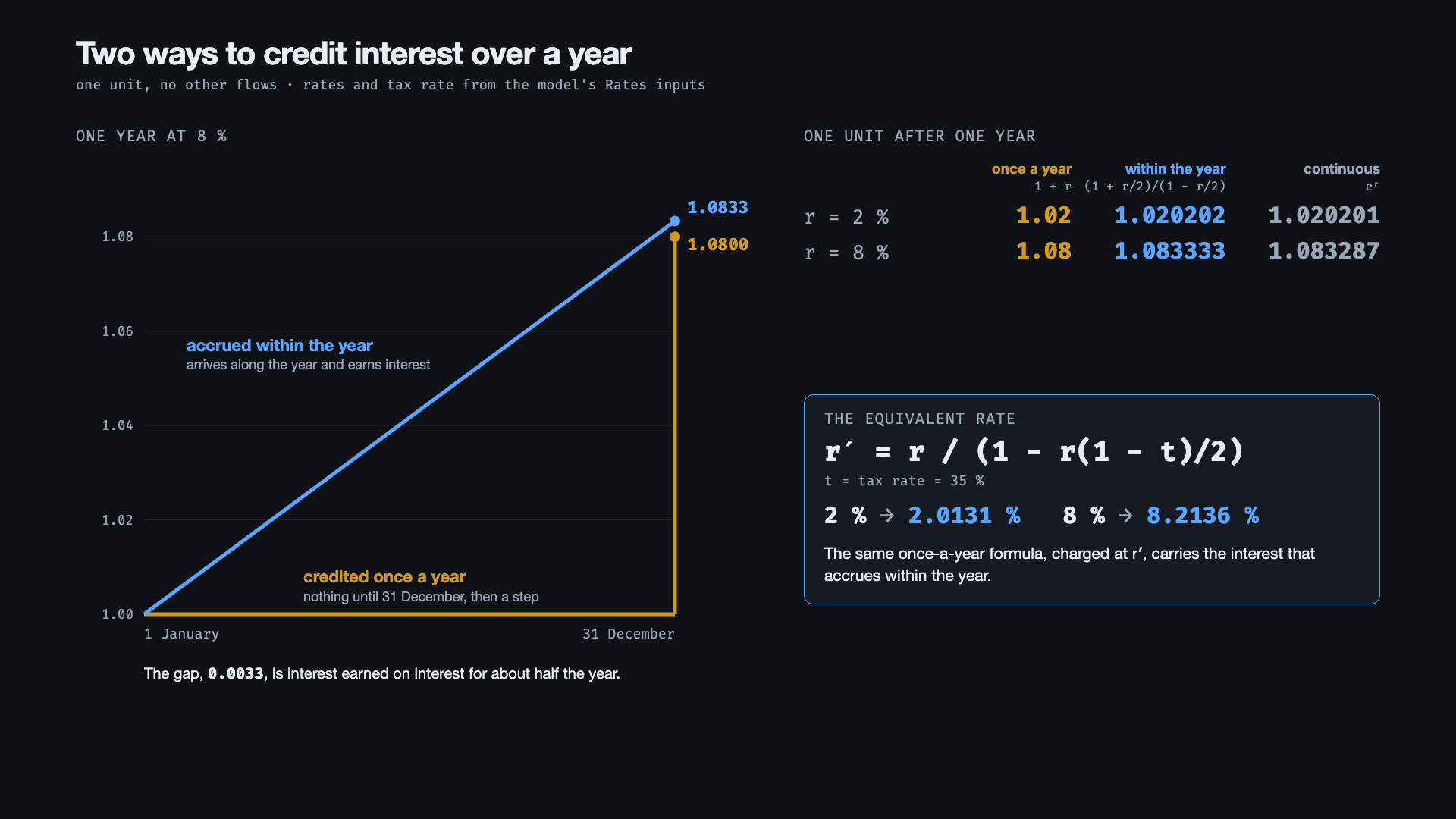
SCF and SCF recursive are two accrual conventions, and neither is an approximation of the other.
In SCF, interest is credited once a year. In SCF recursive, interest accrues within the year and earns interest for about half of it. With no other flows and no tax, a balance a at rate r reaches b with b = a + r\,(a + b)/2, so it grows by
\frac{b}{a} = \frac{1 + r/2}{1 - r/2}
a year, which is a simplified form of continuous compounding. At 2% it gives 1.020202, against 1.02 credited once a year and 1.020201 for e^r. At 8% it gives 1.083333, against 1.08 and 1.083287. The within-year convention is arguably the more realistic one for deposits and overdrafts, which settle interest monthly or quarterly.
The difference between the two statements
A row in SCF measures how far the two statements are apart: Discretionary cash shortfall is discretionary cash in SCF minus discretionary cash in SCF recursive. By year:
| policy | 2023 | 2024 | 2025 | 2026 |
|---|---|---|---|---|
base |
−0.94 | −2.05 | −3.16 | −4.25 |
payout |
−0.88 | −1.78 | −2.62 | −3.38 |
deleverage |
2.44 | 31.72 | 90.97 | 181.18 |
Under base and payout, SCF holds slightly less cash, because it earns no interest on the year’s interest. Under deleverage it holds 181.18 more by 2026, because it charges less overdraft interest, and an 8% overdraft compounds for four years. The numbers are the price of accruing interest within the year.
The equivalent rate, derived
Take one year in which the balance does not cross zero. Let a be the opening balance and b_{BCI} the closing balance before cash interest. In SCF recursive the closing balance includes the after-tax interest, b = b_{BCI} + (1-t)\,I, and the interest is charged on the average of a and b:
I = r\,\frac{a + b_{BCI} + (1-t)\,I}{2} .
Collect I:
I\left(1 - \frac{r(1-t)}{2}\right) = r\,\frac{a + b_{BCI}}{2} \quad\Longrightarrow\quad I = r'\,\frac{a + b_{BCI}}{2}, \qquad r' = \frac{r}{1 - r(1-t)/2} .
The right-hand side is SCF’s formula, the rate times the average of the opening balance and the balance before interest, charged at r' instead of r. At the model’s tax rate of 35%, 2% becomes 2.0131% and 8% becomes 8.2136%.
I asked Claude to put r' into SCF’s two interest lines, without saving. The shortfall under base and payout became 0.00 in every year. Under deleverage it became −1.20, −1.27, −1.33 and −1.40 from 2023 to 2026.
Why the crossing year remains
In 2023 the deleverage balance crosses zero. In that year the average is not the midpoint but the triangle of the closed form, which is quadratic in the closing balance. The derivation above assumed the average was linear in b, and a change of rate cannot reproduce the triangle. The residual of 1.20 appears in that year only. In the following years the balance stays negative, r' matches the interest again, and the 1.20 carries forward at the after-tax overdraft rate: 1.27, 1.33, 1.40. A crossing-year closed form, a quadratic in I, would remove it too. I did not build it.
Two recalculation modes, the same fixed point
Impromptu has two ways to evaluate a cycle group, set per model by recalc_mode. Vectorized, the default, sweeps the group’s datasets whole, in a fixed order, until nothing moves. Granular splits the group into (dataset, line) pieces, orders them by their dependencies, and sweeps those. The setting has no control in the user interface; it is a model setting.
Both modes reach the same numbers. The largest relative difference between their converged values on this model is 2.9e-11, inside the 10^{-10} tolerance.
Where the loop is real, no order computes every line after the lines it reads. The engine has to cut the loop somewhere, and the number of passes depends on where. Granular used to cut it wherever its graph search happened to land: on an earlier engine, 40 different search orders of the same graph gave between 11 and 25 passes on this model. Since an engine change of 2026-09-23 the cut is chosen deliberately, and the count is the same under any search order.
The counts. From a cold start, all three policies together:
base |
payout |
deleverage |
all three together | |
|---|---|---|---|---|
| vectorized | 10 | 10 | 12 | 12 |
| granular | 10 | 9 | 13 | 13 |
The counting rule. Cold means every numeric array of the cycle group {FCF, SCF recursive, BS, IS} set to zero, then the engine’s convergence loop run until the largest relative change between two passes is below 10^{-10}. The count for the whole model is the number of passes the engine runs. The count for one policy is the first pass after which that policy’s largest relative change stays below the tolerance, read from the same three-policy run. The harness that counts them replicates the engine’s loop pass for pass and checks its measure of change against the engine’s own at every pass.
The engine. The counts were measured on Impromptu at commit 4f6e012 (2026-09-23) and reproduced on e8080ee (2026-09-24), which did not change the recalculation code. They describe that engine. A development session scheduled after this post will change the same part of the engine, the ordering of lines inside a dataset; if it moves these counts, this section will be updated with the new numbers and the commit they were measured on.
The counts are not what a user sees at the Recalc button. From a model that is already converged, every recalculation logs 1 pass in both modes. An input edit re-converges from the old fixed point, not from zero: raising the overdraft rate from 8% to 10% under deleverage logs 10 passes vectorized and 13 granular, and both give a 2026 overdraft of 75,228.46. I did not measure wall-clock time; at this model’s size a single run cannot separate the two modes.
The three policies converge together
The three policies live in the same arrays, so the engine converges them together, and the count for the model is the largest over the policies: 12 is deleverage’s 12, and 13 is its 13. The policy that runs an overdraft sets the count for all three, by two passes in vectorized mode. In Excel the iterative-calculation setting is one switch for the whole workbook, so it cannot be set per scenario.
Next: the same model in Excel
Excel can iterate a circular reference, but the setting is one switch for the whole workbook, and a spilled dynamic array cannot take part in a circular reference. This is the first model in the Excel series that needs a fixed point. The next session tries to build it there, with dynamic arrays and LAMBDA and no add-ins, and a post will report what happened.
New episodes go up on the YouTube channel. Everything permanent lives here.
Appendix A, the formulas
Read from the finished model. A bare name is a line of the current dataset; Dataset.name reaches into another dataset; [year:prev] is the previous year and [year:rest] every year but the first. A formula with no qualifier applies to every year and every policy.
SCF, year-end crediting
FCFE[year:rest] = FCF.FCFE
Sale or Purchase of Stock[year:rest] = 0
Dividends = ifelse(FCFE>=0, -FCFE * Rates.dividends pct of FCFE, 0)
Re-add change in operating cash[year:rest] = BS.delta[Minimum operating cash]
NCF BCI = FCFE + Sale or Purchase of Stock + Dividends + Re-add change in operating cash
Net cash position BCI[year:first] = Assumpt.initial total cash
Net cash position BCI[year:rest] = Net cash position[year:prev] + NCF BCI
Discretionary BCI = Net cash position BCI - BS.Minimum operating cash
Excess BCI = ifelse(Discretionary BCI > 0, Discretionary BCI, 0)
Overdraft BCI = ifelse(Discretionary BCI < 0, -Discretionary BCI, 0)
Discretionary prev[year:rest] = Discretionary cash[year:prev]
Avg excess cash[year:rest] = switch((Discretionary prev >= 0) & (Discretionary BCI >= 0), (Discretionary prev + Discretionary BCI) / 2, (Discretionary prev <= 0) & (Discretionary BCI <= 0), 0, (Discretionary prev > 0) & (Discretionary BCI <= 0), (0.5 * Discretionary prev * Discretionary prev) / (Discretionary prev - Discretionary BCI), (Discretionary prev <= 0) & (Discretionary BCI > 0), (0.5 * Discretionary BCI * Discretionary BCI) / (Discretionary BCI - Discretionary prev), 0)
Avg overdraft[year:rest] = switch((Discretionary prev <= 0) & (Discretionary BCI <= 0), -((Discretionary prev + Discretionary BCI)) / 2, (Discretionary prev > 0) & (Discretionary BCI > 0), 0, (Discretionary prev <= 0) & (Discretionary BCI > 0), (-0.5 * Discretionary prev * -Discretionary prev) / (Discretionary BCI - Discretionary prev), (Discretionary prev > 0) & (Discretionary BCI <= 0), (-0.5 * Discretionary BCI * -Discretionary BCI) / (Discretionary prev - Discretionary BCI), 0)
Cash interest income[year:rest] = Rates.excess cash interest rate * Avg excess cash
Overdraft interest expense[year:rest] = Rates.overdraft interest rate * Avg overdraft
Net cash interest[year:rest] = Cash interest income - Overdraft interest expense
After tax cash interest[year:rest] = Net cash interest * (1 - Rates.tax rate)
NCF = NCF BCI + After tax cash interest
Net cash position[year:first] = Assumpt.initial total cash
Net cash position[year:rest] = Net cash position[year:prev] + NCF
Discretionary cash = Net cash position - BS.Minimum operating cash
Excess cash = ifelse(Discretionary cash > 0, Discretionary cash, 0)
Bank overdraft = ifelse(Discretionary cash < 0, -Discretionary cash, 0)
Overdraft warning = ifelse(Bank overdraft > 0, 1, 0)
Total non-cash NWC change = BS.delta[accounts receivable] + BS.delta[raw materials] + BS.delta[finished goods] + BS.delta[other accounts payable] + BS.delta[wages payable]
NCF via cash decomposition[year:rest] = (BS.delta[Minimum operating cash] + (Excess cash - Excess cash[year:prev])) - (Bank overdraft - Bank overdraft[year:prev])
Parity residual B[year:rest] = NCF - NCF via cash decomposition
Cash interest shortfall[year:rest] = Cash interest income - SCF recursive.Cash interest income
Discretionary cash shortfall = Discretionary cash - SCF recursive.Discretionary cash
SCF recursive, within-year accrual
FCFE[year:rest] = FCF.FCFE
Sale or Purchase of Stock[year:rest] = 0
Dividends = ifelse(FCFE>=0, -FCFE * Rates.dividends pct of FCFE, 0)
Re-add change in operating cash[year:rest] = BS.delta[Minimum operating cash]
NCF BCI = FCFE + Sale or Purchase of Stock + Dividends + Re-add change in operating cash
Cash interest income[year:rest] = IS.Interest income on excess cash
Overdraft interest expense[year:rest] = -(IS.Interest expense on bank overdraft)
Net cash interest[year:rest] = Cash interest income - Overdraft interest expense
After tax cash interest[year:rest] = Net cash interest * (1 - Rates.tax rate)
NCF = NCF BCI + After tax cash interest
Net cash position[year:first] = Assumpt.initial total cash
Net cash position[year:rest] = Net cash position[year:prev] + NCF
Discretionary cash = Net cash position - BS.Minimum operating cash
Excess cash = ifelse(Discretionary cash > 0, Discretionary cash, 0)
Bank overdraft = ifelse(Discretionary cash < 0, -Discretionary cash, 0)
Discretionary prev[year:rest] = Discretionary cash[year:prev]
Excess prev[year:rest] = Excess cash[year:prev]
Overdraft prev[year:rest] = Bank overdraft[year:prev]
Swing[year:rest] = Excess prev + Excess cash + Overdraft prev + Bank overdraft
Avg excess cash[year:rest] = ifelse(Swing > 0, 0.5 * (Excess prev + Excess cash) * (Excess prev + Excess cash) / Swing, 0)
Avg overdraft[year:rest] = ifelse(Swing > 0, 0.5 * (Overdraft prev + Bank overdraft) * (Overdraft prev + Bank overdraft) / Swing, 0)
Overdraft warning = ifelse(Bank overdraft > 0, 1, 0)
Total non-cash NWC change = BS.delta[accounts receivable] + BS.delta[raw materials] + BS.delta[finished goods] + BS.delta[other accounts payable] + BS.delta[wages payable]
NCF via Income and BS delta[year:rest] = (IS.Net income - (Total non-cash NWC change + BS.delta[Net fixed assets])) + BS.delta[Financial debt] + Dividends + Sale or Purchase of Stock
Parity residual A[year:rest] = NCF - NCF via Income and BS delta
NCF via cash decomposition[year:rest] = (BS.delta[Minimum operating cash] + (Excess cash - Excess cash[year:prev])) - (Bank overdraft - Bank overdraft[year:prev])
Parity residual B[year:rest] = NCF - NCF via cash decompositionIS, the two interest lines
Interest income on excess cash[year:rest] = Rates.excess cash interest rate * SCF recursive.Avg excess cash
Interest expense on bank overdraft[year:rest] = -(Rates.overdraft interest rate * SCF recursive.Avg overdraft)
BS reads Excess cash, Bank overdraft, Dividends and Sale or Purchase of Stock from SCF recursive. The rest of the model is Episode 2’s.
Appendix B, Glossary
Terms shared with the earlier episodes are defined in the Episode 1 glossary and the Episode 2 glossary. This one adds what is new here.
Discretionary cash, excess cash, bank overdraft
Discretionary cash is the cash balance minus the minimum operating cash the business needs. When positive it is excess cash, earning the deposit rate; when negative its absolute value is the bank overdraft, charged at the overdraft rate.
Accrual convention
When interest joins a balance. Credited once a year, it joins at year end and earns nothing until the next year (annual compounding). Accrued within the year, it joins along the year and earns interest on itself for about half of it.
Equivalent rate r'
The rate at which the once-a-year formula produces the interest of the within-year convention: r' = r / (1 - r(1-t)/2), with t the tax rate. Exact in years where the balance keeps its sign.
Sequential mode
How Impromptu evaluates a dataset with a recursive year dimension: the lines are put in one order, each after the lines it reads, and computed year by year. A line that reads its own current-year result has no place in the order, and the edit that would create it is refused.
Cycle group
A set of datasets that read each other. The engine finds the group and iterates it until no value moves by more than 10^{-10} in relative terms. A cycle group at the level of datasets does not imply a cycle at the level of lines: Episodes 1 and 2 have the first and not the second.
Tolerance and fixed point
A fixed point is a set of values that a further pass leaves unchanged. A converged loop stops when the largest relative change between two passes falls below the tolerance, so its checks read about 10^{-11} rather than zero.
recalc_mode, vectorized and granular
The model setting that chooses how a cycle group is evaluated. Vectorized sweeps its datasets whole; granular sweeps (dataset, line) pieces in dependency order. Both reach the same values within the tolerance, in different numbers of passes.
Parity residuals A and B
Two cash-flow checks. A compares the net cash flow with the one rebuilt from net income and balance-sheet changes; B compares it with the change in excess cash, overdraft and operating cash. Both should read zero, or the tolerance.