Clockwork and dice: a language model where we know every rule
This post opens a new series, the ABC of language models. Each note is paired with a companion video, and each is built around a model small enough to take apart on the bench. Three earlier essays on this blog stand on their own and cover the terminology used here: QKV attention, embeddings and the maps we draw of them, and the final step explain the machinery of a Transformer on models too big to see all at once. This series builds language models small enough to inspect completely, on worlds whose rules we wrote ourselves, so that “did the model learn the rule?” becomes a measurement instead of a guess. The first world is a game I knew by heart as a child. Pietro chiama Paolo (“Pietro calls Paolo”) is a turn-based calling game played around a table. It comes in many variants across Italy, and I would guess well beyond it. We teach it to a language model and then open the model up to see what it made of the rules. Everything here is built and taken apart inside Impromptu, a modeling engine I built from scratch: my own research bench, not a product you can download. Technical terms are explained where first used and collected in the glossary.
This post is the written companion to episode 1 of the series. The video below shows the two models being built, trained and taken apart on the bench. The post is readable on its own.
TL;DR
Most interpretability work is hard because the ground truth is unknown. When a model is trained on a vast natural corpus, what its weights contain has to be guessed from the outside. This series inverts the problem. We invent a small game with explicit rules, generate its dialogues, train a small Transformer on them, and then ask whether the rule is in the trained weights, and if so where.
This first episode does it twice, on two scales:
- Act 1, clockwork. A five-player game with no choice in it: everyone calls the next player in a fixed circle. The whole corpus is one sentence repeated, every round identical. The model memorises it (cross-entropy 0.581 → 0.0012, rule accuracy 1.0 from the first epoch), and we watch end to end how the network turns on the next word: a residual vector is swung until it points almost exactly at one embedding (cosine 0.978), and the readout is a similarity search. This model predicts by position rather than by reading who is calling, and a counterfactual proves it. That is the setup for Act 2.
- Act 2, dice on one decision. Scale to ten players and twelve calls. The machine stays clockwork (a fixed opener, a chain rule, a fixed round length), and randomness enters at exactly one point: whom each player calls. The corpus is now 10,000 rounds, all different, and the loss settles at the entropy of the dice we rolled, 11·ln 9 / 48 ≈ 0.50 nats, measured 0.514, against Act 1’s zero. This model does read the caller. The readout is a spread with the caller pushed to the bottom, the effect follows the caller when we swap them, and the head that attention singles out is not the head that ablation singles out.
The last finding is the reason the toy was worth building. Act 2’s corpus comes from ten formulas, and one of them, a single comparison and a single addition, is the whole “don’t call yourself” rule. The trained model matches those formulas’ output on both measures we can check: distribution (loss within a hundredth of a nat of the computed floor) and behaviour (rule accuracy exactly 1.0). The results are equivalent. The machinery is nothing alike. We found the part that does the copy. We never found a part that is the rule. Removing the single most causal head still leaves rule accuracy at 0.86. On the easiest interpretability problem anyone could construct, we can prove the rule is in there and still cannot point at it.
One methodological point runs through both acts. The optimiser minimises one quantity, cross-entropy. Learning the rule happens, or fails to happen, only insofar as the rule coincides with the statistics.
The glossary explains the terms in those bullets. The long version follows.
Act 1, the clockwork game
The game, and the circle
Five players: Pietro, Paolo, 1, 2, 3. There is one rule and no choice at all. Each player calls the next one along a fixed circle,
\text{Pietro} \to \text{Paolo} \to 1 \to 2 \to 3 \to \text{Pietro},
and when the call comes back round to Pietro the round is over. Every round is the same five calls, written in the model’s token encoding as:
<BOS> Pietro chiama Paolo <SEP> Paolo chiama 1 <SEP> 1 chiama 2 <SEP>
2 chiama 3 <SEP> 3 chiama Pietro <EOS>
chiama is Italian for “calls”. The vocabulary is nine meaningful tokens (the five names, chiama, and the three markers <BOS> / <SEP> / <EOS>) plus a padding token, ten slots in all. A round is 22 tokens, so a context window of 24 holds it comfortably. At this scale both concepts are visible: a small vocabulary and a short context window are things one can hold in mind, before we scale them up and they become abstractions.
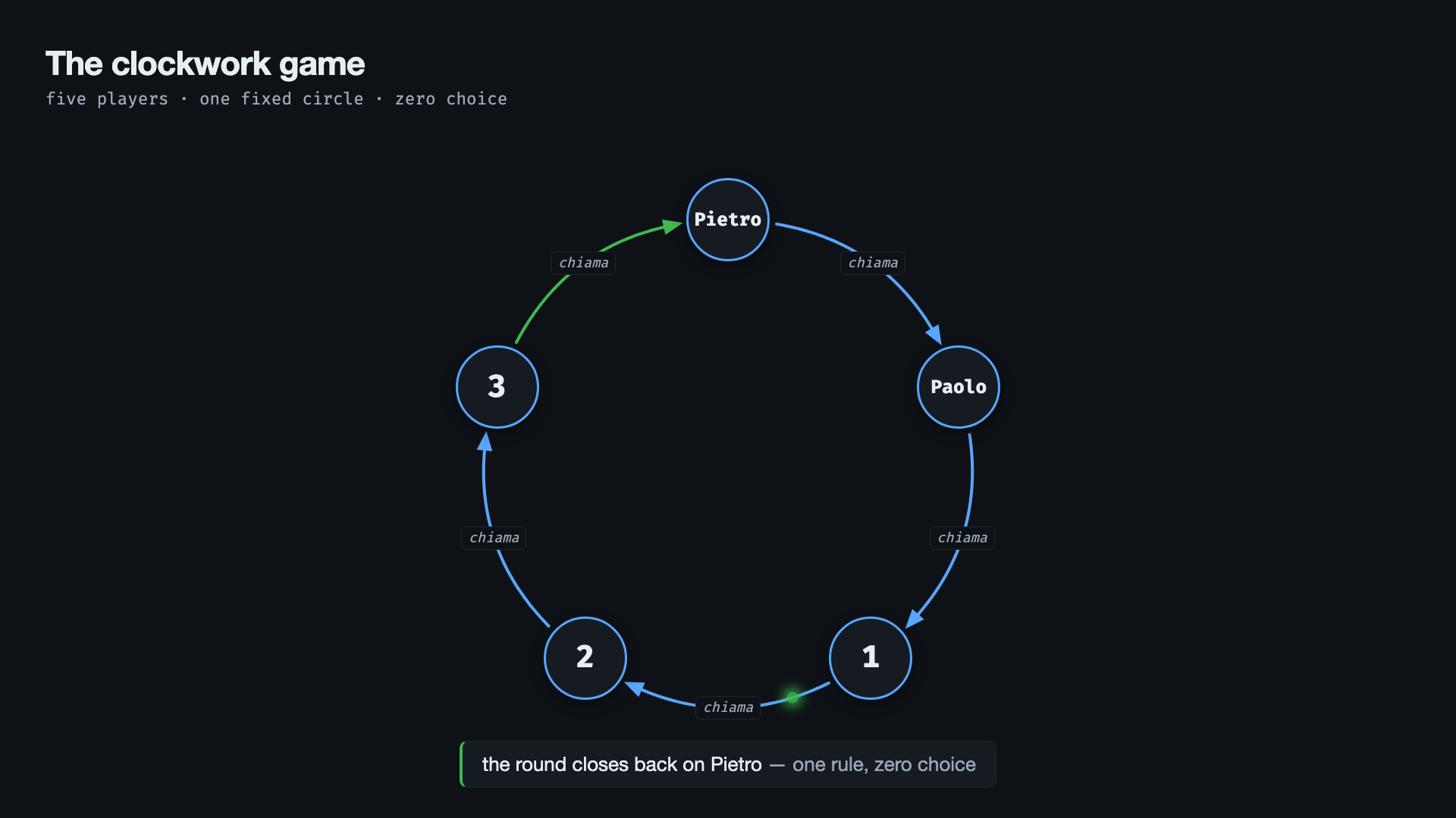
chiama arrow from each to the next and the last arrow closing the round back on Pietro. One rule, no choices.The corpus is the rule, played out
There is no corpus generator to distrust, because the rule is the whole generator. We defined a five-player circle, and a single seeded action plays that rule out and writes the games straight to text: one button, the same corpus every time. There is no hidden state and no second model producing the data. The corpus is the rule we wrote, spelled out in full.
That is the point of the series. We authored the rule ourselves, so we know the ground truth with certainty, and “did the model learn it?” is a measurement. (How the model is built and laid open, as a Transformer represented as a grid of cells one can select and edit, is its own story, told in a companion note.)
Uniform on purpose
Every round is the same sentence. Scroll the corpus and the rows are identical, top to bottom. A language model trained on this can only memorise. That is deliberate. Act 1 is the control experiment, the world with no randomness at all, so that everything the model does is legible.
The Transformer we train on it is oversized on purpose: roughly 100,000 parameters (two layers, four attention heads each, embedding dimension 64) to represent a successor table that fits in five cells. We use the oversized machine to watch how it represents a rule that does not need it. (On ancestry: a bigram table, which counts which token follows which and is itself computed by formula from the corpus, already predicts this game perfectly, since the bigram’s most likely next token is the successor function. N-gram language models did this for decades. This series is about the Transformer’s internals rather than the n-gram baseline.)
The score we train against is cross-entropy, a score for a probabilistic forecast. At each step the model does not name a single next word. It spreads a probability over all possible next words, and cross-entropy looks only at the probability it placed on the word that actually came next, penalising it for whatever was missing from 100%. The penalty is largest when the model was both confident and wrong. It is the same log score a statistician uses to rate a weather forecaster, or a default-probability model graded on how much probability it put on the names that actually defaulted. It is the appropriate way to keep score when the answer is a distribution rather than a single pick. (The formula, −log p, is in the glossary.)
That score becomes a trained model in the same way an econometrician fits a model by maximum likelihood: choose the parameters that make the observed outcomes as probable as possible, which is the same as minimising −log p on those outcomes. A linear regression is solved in closed form, and a logistic default-probability model is fitted in a handful of Newton steps. Here there are ~100,000 weights and no closed form, so the fit requires a long iteration. The training rounds are pushed through in small batches. For each batch the model computes its average cross-entropy and then computes, for every weight, the direction in which a small change would make the loss smaller. That direction of steepest descent is the gradient, and the model takes one small step along it. The size of the step is the learning rate. Then the next batch, another step, and so on. One full sweep through the training data is an epoch. Each epoch is hundreds of these steps, and after each epoch we score the model on a held-out validation split it never trained on. Those validation scores are the numbers below. Over epochs the steps drive the loss as low as the data permits and then stop making headway, and the curve flattens on its floor.
Here the score falls essentially to zero, 0.581 → 0.028 → 0.0125 → … → 0.0012 over twelve epochs, and there is no floor, because the corpus has no randomness to be uncertain about. Rule accuracy is 1.0 from the first logged epoch. Memorisation is instant, so the only curve worth watching here is the cross-entropy tail. In Act 2 the loss will settle at ≈ 0.50 nats and go no lower. That is the entropy of the one free choice the game leaves to chance, and the contrast with Act 1’s zero is the lesson.
The residual-stream walk, how the network turns on the right word
The centrepiece of Act 1 is how the network turns on the next player. On a model this small we can watch it end to end, in the glass box, with the logit lens (on camera, from 4:19). The walk has three pieces.
- Embedding, a token as a location. Every token is stored as a 64-number vector learned during training. It can be pictured as a point, or a direction, in a 64-dimensional space: the token’s meaning expressed as a place. Because in this model the input and output embeddings are tied, that same location is also how the model names the token when it produces output.
- Residual stream, a workspace built up in steps. As the model reads, it keeps one running 64-number vector per position, a scratch workspace. Each attention head and each feed-forward block adds a correction to it. Nothing is overwritten. The contributions accumulate, and by the end this workspace is the model’s whole summary of what should come next at that position.
- Readout, scoring each word by alignment. To turn that workspace into a next word, the model measures how far the workspace points the same way as each token’s embedding. The measure is a dot product, the basic agreement number between two vectors, larger when they point together. One such number per vocabulary word is that word’s logit. The softmax (exponentiate, then normalise so they sum to 1) turns the logits into probabilities. The output step is a similarity search for the stored location closest to the workspace.
At the position right after chiama, each write the trained model makes moves the workspace a little further toward Paolo’s location. Measured after each block write, the alignment (the same dot product) with Paolo’s embedding climbs, snapshot by snapshot:
0.08 \;\longrightarrow\; 2.75 \;\longrightarrow\; 4.45 \;\longrightarrow\; 6.07 \;\longrightarrow\; 8.15.
That growing number is Paolo’s logit, built up one write at a time. The final value, 8.15, is the score Paolo carries into the softmax.
On the probe <BOS> Pietro chiama, the successor comes out Paolo @ 0.9986, one bar near 1 in the full ten-way softmax, because the workspace ended up almost exactly parallel to Paolo’s embedding. There are two ways to state that. The raw alignment, Paolo’s logit, is 8.15, far above every rival. The cosine is the same alignment stripped of length, so it reads as a pure angle, 1.0 meaning identical direction and 0 meaning perpendicular. Here it is 0.978, with every other token near-orthogonal (cosine ≤ −0.13). The phrase “the direction pointing at the following player is turned on” is literal here: \text{logit}(t) = h \cdot e_t, and the workspace h has been swung until it points at exactly one embedding e_t.
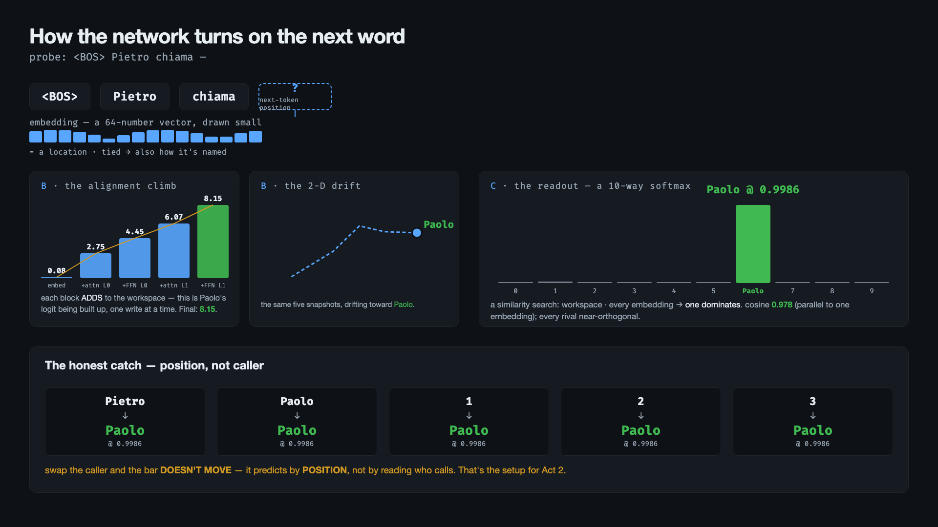
<BOS> Pietro chiama —. Left: the alignment climb, Paolo’s logit built up one additive write at a time: 0.08 at the embedding, then 2.75, 4.45, 6.07, 8.15 after each attention and feed-forward block. Middle: the same five snapshots as a drift in two dimensions, the workspace migrating toward Paolo. Right: the ten-way softmax that reads the workspace out, one spike, Paolo at 0.9986, cosine 0.978. Below: swap the caller and the bar does not move. Pietro, Paolo, 1, 2, 3 all give Paolo at 0.9986. The model predicts by position, not by reading who calls.This model predicts by position, not by caller
It would be easy to narrate the readout above as “the model reads that Pietro is calling and answers Paolo.” It does no such thing. Swap the caller and the prediction never moves: <BOS> X chiama gives Paolo for every X, even 1 chiama → 1. The uniform corpus handed the model a shortcut (position 4 is always Paolo), so there is no caller-binding here, and no attention-versus-causation story to tell. The causal head carries a positional readout, not a read of who is calling.
A shortcut by position is available because position is itself written into the workspace. Before the first layer, every token’s embedding has a positional encoding added to it: a fixed pattern of the same length as the embedding, different for every slot in the sequence (the glossary has the intuition). So the vector that enters the network at the fourth slot says both “this is chiama” and “this is the fourth slot”. A model is free to read the second half alone and answer Paolo, and on a corpus where the fourth slot is always followed by Paolo that is the cheapest thing to learn.
That is the setup. Reading who is calling only becomes necessary when the answer is not fixed, which is what Act 2 supplies.
Act 2, scale the clockwork and roll dice on one decision
The same machine and a bigger game, still clockwork
Ten players now (Pietro, Paolo, 1–8), rounds of twelve calls, and one permissive rule: call anyone except yourself. Almost everything stays deterministic. The engine hard-codes the opener, so every round begins <BOS> Pietro chiama Paolo. The chain rule fixes each caller: whoever was just named calls next. The round ends after exactly twelve calls. The players are error-free (p_correct = 1.0), with no self-calls and no nonsense. The randomness lives in exactly one place, the callee after each chiama, drawn uniformly among the nine players other than the caller.
The corpus comes from the same action as Act 1, the same button, now with one random draw per call. That draw has to be seeded. A naive random() would re-roll on every recalculation and give a corpus that cannot be reproduced, so the action fixes the seed and returns the same 10,000 rounds every time. In Act 1 the button wrote one sentence over and over. Here it writes ten thousand different ones. Everything around that one draw is still fully determined.
The rules, written down as ten formulas
The action wrote the corpus. The rules themselves are what the trained model is held up against at the end of this post, so they are written out here. A CorpusCalc dataset reconstructs the corpus from formulas alone, in ten lines. Three of them carry the whole game:
caller_pos[call:rest] = callee_pos[call:prev]         # the chain rule
draw                  = dg_seeded_draws(42)           # the dice, replayed
callee_pos[call:rest] = draw + (draw >= caller_pos)   # "call anyone except yourself"
The first is the chain rule: whoever was just called is the next caller. The second replays the same seeded stream of nine-way draws the generator rolled. As in the action, the formula may not call random(), which would re-roll on every recalculation, so the dice arrive as a seeded function and recalculating is idempotent. The third line is the entire no-self-call rule. Number the draws 1…9 and step up by one as soon as the count reaches the caller’s own seat, so that the nine draws land exactly on the nine players who are not the caller. That is one comparison and one addition. There are zero self-calls in 12,000 generated cells, by construction rather than by luck.
The remaining seven formulas are bookkeeping: chiama is a constant, the separator is decided by position, two lookups turn seat numbers into names, and one line glues the tokens into text. The shape of the world is explicit in them. Of the four tokens in every call, three are forced and exactly one is drawn, and the first call is not even that, since the opener is fixed. Run the ten formulas and they reproduce the first 1,000 training rounds byte for byte, string-identical to what the action wrote.
Being a replica of the action-generated corpus, CorpusCalc is never used for training. It exists so that at the end there is a small set of exact formulas to compare the weights against.
Vocabulary and context grow for visible reasons: ten names, sequences of 1 + 12×4 = 49 real tokens, a window of 80. Both are still small. The corpus is no longer uniform. Scroll it and all 10,000 rounds are different, because that one free choice compounds across the eleven calls after the opener. Memorising individual sentences is now useless. The model must compress the one distribution that repeats.
The grammar walk, scaffold at ~100 % and one choice at ~ln 9
This is the clearest single demonstration in the episode (read off cell by cell, from 9:52). Walk one round position by position and read off, at each step, the model’s top-1 prediction, its probability, and the entropy of its whole distribution (a Grammar dataset does this cell by cell). Entropy is a one-number measure of how spread out a set of probabilities is, in the same log units (nats) as cross-entropy: how many equally likely options the model is hesitating among. It is zero when the model is certain, with all the probability on one token, and ln k when it is torn evenly among k choices. A fair nine-way pick has entropy ln 9 ≈ 2.2 nats. (Formula in the glossary.) The deterministic scaffold is predicted with near-total confidence, ≥ 0.996 with near-zero entropy at every step:
| position type | what the model must predict | prediction |
|---|---|---|
<BOS> → |
the fixed starter | Pietro |
the fixed opener Pietro chiama → |
Paolo, always | 1.000 |
| a name → | chiama |
≥ 0.996 |
| a callee → | <SEP> |
≥ 0.996 |
the chain rule <SEP> → |
the previous callee | 0.996 |
| after call 12 → | <EOS> |
1.000 |
Exactly one position type is uncertain: the callee right after chiama. There the entropy sits at ≈ 2.25 nats = ln 9, a uniform hesitation over the nine valid targets. There are eleven such positions per round, and everything else is pinned. This is the same fact the ten formulas state from the outside (three tokens forced, one drawn), now measured from the inside, by the model, without our having told it. Conditional probability changes with the step in the turn and the turn in the game, and on this toy that can be read straight off a spreadsheet, cell by cell.
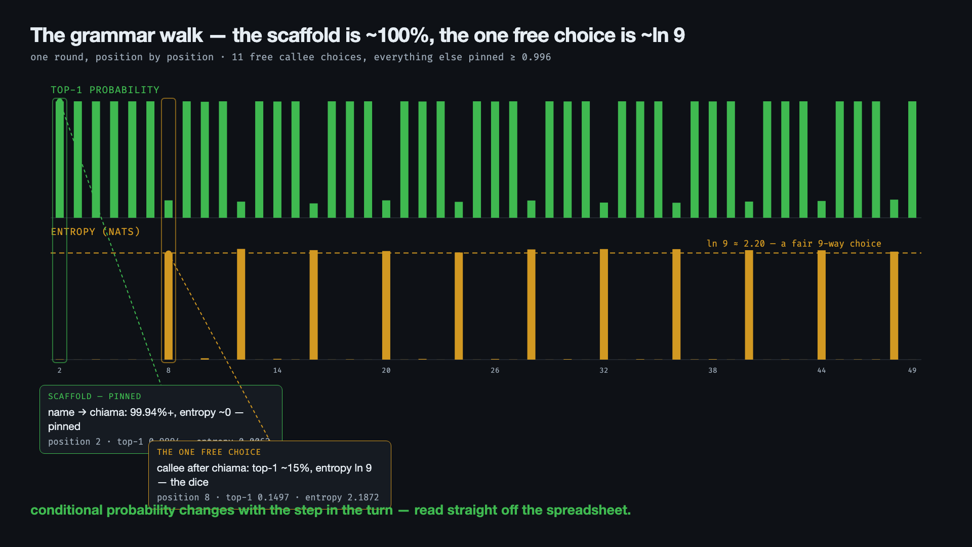
chiama, every separator) is pinned at 99.94 % and entropy ≈ 0. Eleven positions break the pattern: the callee after each chiama, where top-1 drops to ≈ 15 % and entropy rises to the dashed line at \ln 9 \approx 2.20, a fair nine-way choice. The dice are struck eleven times.The loss settles at the entropy of the dice
Cross-entropy makes a fast marginal descent, 2.14 → 0.514. Rule accuracy climbs from 0.083 to 1.0 (by epoch 27), but not monotonically. It dips −0.056 by epoch 7, when the confident marginal argmax lands on the recent caller, the one forbidden answer, before the circuit that suppresses it has formed. In the tail the two decouple: from about epoch 21 the loss sits almost flat on its floor (~0.52) while rule accuracy is still climbing, 0.987 → 1.0.
“Almost flat” is a statement about the scale of the chart, and it is worth reading the log at more decimals. From epoch 21 to epoch 50 the validation loss goes 0.5366 → 0.5325 → 0.5298 → 0.5288 → 0.5282 → 0.5268 → 0.5264 → … → 0.5146: about 0.022 nats in thirty epochs, a thousandth of a nat per epoch, against 1.08 nats in the first three epochs. Over the same thirty epochs rule accuracy climbs from 0.987 to 1.0. The optimiser never stops descending; nothing in it recognises a floor. The contrast between the two curves is between orders of magnitude of change, not between change and no change. That the last hundredths of a nat pay for the last points of rule accuracy is the whole point of the next section, and next episode the same arithmetic runs the other way: a change of under a thousandth of a nat in the loss flips the model’s best guess.
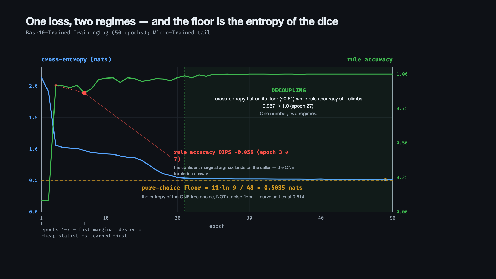
In the clean game the floor is exactly computable. Each of the eleven free callee choices per round is uniform over nine valid targets and contributes ln 9 of irreducible entropy. Spread over the 48 scored positions in a round,
\frac{11 \cdot \ln 9}{48} = 0.5035 \text{ nats}.
The trained model settles at 0.514, slightly above the floor and no lower. The loss goes as low as the irreducible entropy of the one free choice, and no further. Set against Act 1’s zero floor, the lesson is that a language model’s loss floor is the entropy of whatever its corpus left to chance. (There is no noise floor here, because no dice break the rule. That arrives next episode.)
Why the curve has that shape, the dip and the decoupling
That shape invites a wrong reading: two competing objectives inside training, a statistical one that fits the token frequencies and a rule-based one that obeys the game, taking turns. There is one objective. Cross-entropy is the only thing being minimised. Rule accuracy is never part of the loss. It is a behavioural measurement we compute from the outside, because we own the simulator and know the ground truth. The model is never told the rule and never rewarded for it, and it holds no representation of the rule as a goal. What the curve shows is two ways the one loss can be driven down, and the cheaper way is taken first.
Marginal statistics, the cheap win. Learn which tokens are frequent where: after
chiamacomes a player’s name, after a name comeschiamaor<SEP>, after<SEP>a name again. Getting the right kind of token into the right slot accounts for most of the loss for almost no effort, which is why it produces the big early drop. A small Transformer like ours starts close to a copy machine: with tied embeddings its untrained tendency is to repeat a recent token, and copying is a decent marginal strategy here, because the next token usually is something seen a moment ago. The copy tendency has a side effect. At a decision position,… Paolo chiama 4 <SEP> 4 chiama —, the most recent name is4, the caller, so the copy-biased guess is4, a self-call and the one forbidden answer. That is the dip: rule accuracy falls while cross-entropy is still dropping fast.The loss does punish that, and the punishment is what eventually fixes it. Cross-entropy scores only the probability placed on the token that actually came next, and in this clean game the real next token is always a valid callee, never the caller. Every scrap of probability the copy tendency spends on
4is probability not spent on the callee that occurs, so −log p on that position goes up. The penalty is tolerated at first because the arithmetic favours it: the self-call mistake costs a little loss, while getting the overall token-type distribution right gains a lot, so steepest descent takes the big marginal win first and removes the small self-call penalty later.Contextual computation, paying down the rest. “Later” means building a circuit: attention that looks back, reads who the caller is, and pushes that one token’s logit down so the freed probability flows to the nine valid callees. This is the expensive part, learned last, and it moves the loss only a little, because the marginals already captured most of it. That is the decoupling after epoch 21: cross-entropy is already sitting on its floor while rule accuracy still has 0.013 to climb. The optimiser was never told the rule. The suppression circuit forms because suppressing the caller is what removes the last sliver of wasted probability.
The two act in succession because of gradient economics, not by design: the cheapest descent comes first. The log puts numbers on the prices. The first three epochs remove 1.08 nats of validation loss (2.142 → 1.058), and rule accuracy reaches 0.919, close to the nine in ten that any name chosen without regard to the caller would score. The whole no-self-call rule, by contrast, is worth at most (ln 10 − ln 9) · 11/48 ≈ 0.024 nats: the difference between spreading probability over ten names and over the nine valid ones, at the eleven free positions of the 48 scored. That is the size of the tail descent, 0.022 nats from epoch 21 to 50. The logged gradient norm follows the same order: 0.38 at epoch 1, down to 0.13 by epoch 6 once the cheap statistics are in, and between 0.2 and 0.5 for the whole tail, where the remaining gradient is the small self-call penalty. Between the two phases the log shows a third movement that the chart compresses: from epoch 15 to epoch 20 the validation loss falls from 0.817 to 0.545, 0.27 nats, and the gradient norm, under 1 before, rises to 7.2 at epochs 17 and 18 before settling. That is most likely the chain-rule copy forming, the circuit L0H3 carries: knowing the next caller is worth ln 10 at eleven of the 48 positions, about 0.5 nats, far more than the rule and far less than the marginals. The rule gets learned at all only because, in this clean world, the rule-respecting prediction is also the loss-optimal one. No player ever violates the rule, so the statistics and the rule coincide exactly, and learning the one is learning the other. That identity is conditional. Noise breaks it, and noise is where the series goes next.
Interpretability at a mid-round call
Because the opening is deterministic, the interesting binding is at a mid-round decision. Take … Paolo chiama 4 <SEP> 4 chiama —, where the model must predict whom 4 calls. To get it right the model must read who the caller is and push that one name down. Everything below is measured on this trained model. The head indices are this model’s own: they come out of the random seed, and a different seed would in general place the circuit differently.
1. The readout is a spread, and the caller is at the bottom. Dotting the residual stream against every embedding no longer gives one dominant direction. It gives a spread over the nine valid callees, with the caller 4 driven to the bottom (rank 10 of 10, probability 0.006, cosine 0.417, parallel to no single embedding). This is the mirror image of Act 1’s single-embedding spike (cosine 0.978). The clockwork model memorised a position. This model reads a name.
2. The counterfactual follows the caller. Swap the caller, … Paolo chiama X <SEP> X chiama, and that name, whichever it is, gets suppressed, for 9 of 9 callers, with the top pick never the caller. (In Act 1 the prediction never moved.) There is no Pietro exception here. The fixed starter is special only at the opening position, not mid-round. The binding is to content, not to position.
3. Probe A, attention (correlation). Read the caller-attention of every head. One head, L0H1 (layer 0, head 1), stands out, with 0.72 of its attention on the caller. By inspection it is a textbook rule head, the kind of picture the Transformer paper offered when it reported that “individual attention heads clearly learn to perform different tasks” and that many “appear to exhibit behavior related to the syntactic and semantic structure of the sentences” (Vaswani et al., Attention Is All You Need, 2017).
4. Probe B, ablation (causation). Remove heads one at a time and re-measure the rule. Removing L0H1 barely moves it (Δ −0.031). L0H3, with caller-attention of only 0.087, is the head whose removal breaks the rule most: Δ rule accuracy −0.140. A head’s attention shows what it reads, not what it does, and only removal and re-measurement separates the two. (Both probes, side by side, from 14:07.)
5. The ablation as a cell edit, on the chain-rule copy. The cleanest thing to break by hand is not the distributed suppression, which is soft and spread over nine tokens, but the deterministic copy beside it. At … Paolo chiama 4 <SEP> —, the next caller is the callee just named, 4, predicted at 0.999 by attending back and copying it. In the glass box, select L0H3’s output block in the W_o weight matrix, zero it, and press Recalc. The copy flips to a wrong token, 4 → 2, and p(4) collapses 0.999 → 0.0005. The rule is broken by hand, in a top-1 flip as unambiguous as Act 1’s. (On camera, from 12:31.) Zero an inert layer-1 head (L1H2) instead and 4 holds at 0.999. Causality is tested by hand, in a spreadsheet.
L0H3 is the same head that suppresses the caller at the free choice. One head reads the relevant earlier name, to copy it here and to suppress it there. One circuit does two jobs. (The copy is the on-camera demonstration and the suppression is not, because the copy is a single sharp top-1 flip, whereas the free-choice suppression is distributed across the spread and moves softly under ablation. That is the contrast between one memorised circuit and one distributed rule.)
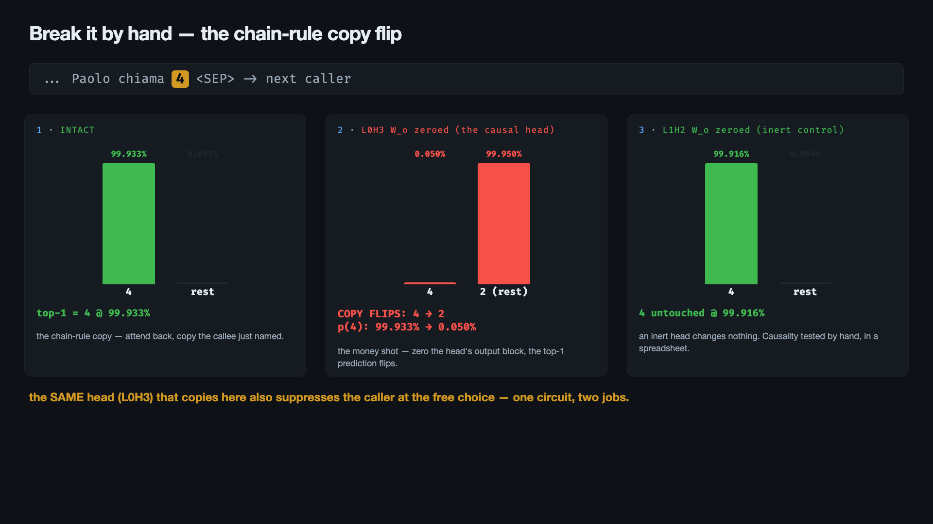
… Paolo chiama 4 <SEP> →. Left, intact: the chain-rule copy, 4 at 99.933 %. Middle, L0H3’s W_o block zeroed: the top-1 prediction flips to 2 and p(4) collapses to 0.050 %. Right, the control: zeroing an inert head, L1H2, leaves 4 at 99.916 %. The causality is tested, not assumed. The same head that copies here also suppresses the caller at the free choice, one circuit doing two jobs.Equivalent results, alien machinery
The comparison the toy was built for is between the two halves of this post (the episode ends on it, at 17:44). On one side, ten formulas. On the other, a trained model of about 107,000 numbers. By both of the measures we can check, the model came out equivalent to the process that wrote its data.
Distributionally. Cross-entropy settles at 0.514 against a floor we computed from the generator, 0.5035. The comparison rests on a decomposition. Expected cross-entropy splits exactly into H(p) + D_{KL}(p\,\|\,q): the irreducible entropy of the true process, plus the divergence between the model’s conditional distribution and the true one. The floor is H(p), so the gap between the two numbers is the KL divergence, about a hundredth of a nat. The loss is near enough the entropy, so the distribution is near enough matched.
Behaviourally. Rule accuracy is exactly 1.000 on held-out rounds: across every scored decision, the model’s top token is never the caller. The hard constraint that took one comparison to write is honoured without exception.
Same distribution, same hard constraint: the results are equivalent.
Nothing about the machinery is equivalent, and there was never a reason to expect it to be. A Transformer is a general architecture rather than a rule compiler, built so that some setting of its weights can represent, under size and complexity constraints, almost any language world it might be trained on, driven by an optimiser with one instruction: make the cross-entropy smaller. Nothing in that arrangement aims to put our one-term rule anywhere we could find it. The architecture is far more expressive than the small world it was handed, and it uses that expressiveness however gradient descent found convenient.
That is visible in what we found and in what we did not find:
- We found the copy. The chain rule (whoever was just named calls next) has a crisp implementation. L0H3 attends back and copies. Zero that head’s
W_oblock and the prediction flips4 → 2, withp(4)collapsing 0.999 → 0.0005. It is a rule-shaped part doing a rule-shaped job. - We never found the rule. “Call anyone except yourself” has no such part. Ablate each of the eight heads in turn: the largest single effect is that same L0H3 at Δ −0.140, which still leaves rule accuracy at 0.860. All four layer-0 heads carry a piece (−0.031, −0.040, −0.140, −0.082), and the four layer-1 heads register nothing at all. There is no head whose removal switches the rule off.
Two qualifications apply to the negative result. First, “we never found it” means precisely: no single head, under single-head zero-ablation. We did not search head pairs, feed-forward neurons, or directions in the residual stream, and a determined circuit hunt might well localise more than we did. Second, the rule is in there and it is causal: swap the caller and the suppression follows the new caller, 9 times out of 9. The finding is that the rule is not localised to anything we could surgically remove. It is spread across parts, and it shares those parts with other work. L0H3 copies the chain token here and helps push the caller down there, one circuit with two jobs.
That result generalises past this toy in an uncomfortable direction. This was the easiest case anyone could construct: a world whose ten rules we wrote ourselves, a model small enough to print, ground truth in hand, and every weight in a spreadsheet cell we could select and zero. We can measure that the model implements the rule, we can prove causality by breaking it, and we cannot point inside and say where it is. Interpretability worked here, and it did not hand back the formula.
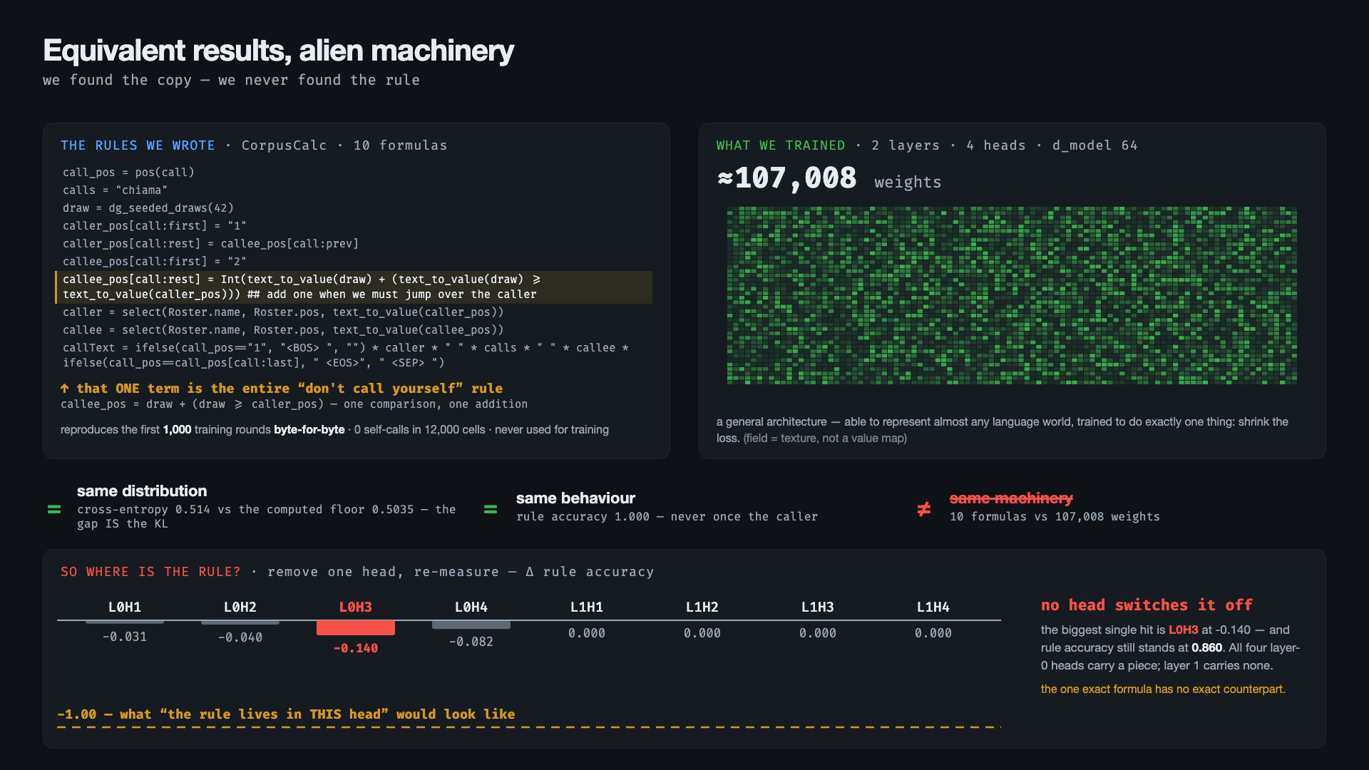
A note on lesions, Phineas Gage and how far ablation carries
The move we just used (remove a part, re-measure the behaviour, infer what the part was for) is old, and it comes with a long-running lesson about how far that inference carries.
In 1848, a railway construction foreman in Vermont named Phineas Gage survived a tamping iron blown up through his left cheek and out of the top of his skull. His movement, his speech and his memory came through. His character, by the accounts that followed, did not. His physician John Harlow reported that acquaintances found him profane, capricious and unable to hold to a plan, and said that he was “no longer Gage.” A century and a half later, Hanna Damasio and colleagues reconstructed the rod’s path from Gage’s preserved skull and placed the damage in the ventromedial prefrontal cortex (Science, 1994). Antonio Damasio built on patients of this kind in Descartes’ Error to argue that emotion is part of the machinery of reasoning rather than its opponent.
That is a lesion study, which is to say an ablation. What it delivered and what it did not deliver should be stated precisely. It established that a region is necessary for a class of behaviour. It did not show that the region contains that behaviour, did not explain how the behaviour is produced, and did not predict what a different patient with similar damage would look like. The story also got tidier in the retelling than the evidence supports: the historian Malcolm Macmillan has traced how much of the familiar version accumulated after the fact, and Gage appears to have recovered considerably. He spent years driving coaches in Chile.
Every one of those caveats transfers unchanged to zeroing a block of W_o and re-measuring rule accuracy. Ablation establishes necessity, not location. The story it supports is always neater than the mechanism. A redundant, distributed system tolerates the removal of any single piece, which is what our eight bars show, with the tallest of them leaving 86 % of the rule intact. Damaging one specific part changes behaviour in a way we can measure precisely and cannot explain. That is the state of play for a brain. On the easiest example anyone could build, it turned out to be the state of play for a hundred-thousand-parameter Transformer as well.
What the toy bought us
The toy bought us ground truth. Every claim above was checkable because we wrote the rules ourselves: a uniform corpus generated from a fixed circle in Act 1, and in Act 2 ten formulas with exactly one free choice in them, a clean world on purpose. We computed the cross-entropy floor from the corpus geometry and watched the model settle onto it. We removed the head and watched the rule fall, instead of reading a rule head off an attention picture.
It also bought us one thing we did not go looking for, a negative result we can trust. “The model did not localise the rule” is an empty sentence on a natural corpus, where nobody knows what the rule was. Here it is a measurement, because we can hold the ten formulas in one hand and the ablation bars in the other. The model reproduces our world almost exactly, with machinery that looks nothing like the rules we wrote.
Next in the series, the dice violate the rule at a known rate, and the loss-optimal predictor turns anti-rule past a closed-form threshold. After that come games where the valid answer depends on who is speaking.
See it happen in the companion video
Every claim in this post is shown in the companion video (embedded at the top), on the trained models themselves: the residual-stream walk swinging the workspace onto Paolo, the grammar walk read off cell by cell, the mid-round readout going from spike to spread, and the copy-flip ablation, where zeroing one attention head’s weights by hand flips the model’s top prediction from 4 to 2 on camera, after which an inert head leaves it untouched. The ten CorpusCalc formulas are on screen too, alongside the ablation bars, for the comparison the episode ends on.
That is possible because the whole thing lives inside Impromptu, a modeling engine I built from scratch, where a formula reads caller → callee rather than =B7*C7 and the network’s weights are datasets like any other. A block of a weight matrix is a range one can select and set to zero while the prediction updates in the cell beside it. Impromptu is my own research bench, not a product you can download. The video is the window onto it. The dialogue game these two models learn, Pietro chiama Paolo, is the ToyDialogueGames exercise.
Glossary
For readers who want the basics or a refresher.
Token, vocabulary. A token is the unit the model reads, here a whole word. The vocabulary is the finite set of possible tokens. Act 1’s has nine meaningful tokens (five names, chiama, and the markers <BOS> / <SEP> / <EOS>) plus <PAD>. Act 2 adds five more names.
Causal language model. A model that, given a sequence, predicts the next token having seen only the previous ones, never the future. Prediction at position t uses positions 1…t only. GPT-style models are all causal in this sense.
Transformer. The neural-network architecture whose key ingredient is attention: at every position the model can look back at every earlier position and weight how much to pull from each. It is a stack of identical layers, each an attention sub-layer then a feed-forward sub-layer, each wrapped in a residual connection. For the mechanistic reading used here, Christopher Olah’s Transformer Circuits Thread and Anthropic’s A Mathematical Framework for Transformer Circuits are the two most accessible references.
Layer, attention head. A layer is one pass of (attention, feed-forward, residuals). Our models have 2. Inside attention the work is split across heads, parallel sub-attentions, each with its own pattern of which positions to attend to. We have 4 heads per layer, 8 in total. Identifying which head does what is the central activity of mechanistic interpretability. (We write L0H3 for layer 0, head 3; layers are numbered from 0.)
Embedding, tied embedding. Each token is represented as a vector of real numbers (here 64-dimensional). The input embedding maps a token id to its vector. The output projection maps the model’s final vector back to a score per vocabulary token. Tied means the two are the same matrix: the model names a token with the vector it reads it as. This is why the readout is a similarity search. Before the first layer a positional encoding is added to each token’s embedding: a fixed vector of the same length, built from sines and cosines at a range of frequencies, so that every slot in the sequence gets a different pattern. The vector that enters the network therefore carries both the token’s identity and its position, and a model can attend to or predict from either. The clockwork model predicts from the position alone.
Residual stream. The running tape of vectors a Transformer maintains, one per position. Each attention and feed-forward output is added to it. Components write into the residual stream, and nothing is overwritten. Watching which component writes what is the core of the Act-1 walk.
Logit, softmax, argmax. The model’s raw output per position is a vector of |vocab| real numbers, the logits. Softmax turns them into probabilities (exponentiate, divide by the sum). The argmax is the index of the largest, the model’s single best guess. Here, \text{logit}(t) = h \cdot e_t: the dot product of the workspace with token t’s embedding.
Entropy, nats. A one-number measure of how uncertain a probability distribution is: H = -\sum_i p_i \ln p_i. It is 0 when one outcome has all the probability (no uncertainty) and ln k when k outcomes are equally likely, the uncertainty of a fair k-sided die. Measured in nats when the logarithm is natural (in bits with log base 2). Intuitively, entropy is the number of equally likely options one is effectively choosing among, in log units. In Act 2 the callee is a fair nine-way choice, so its entropy is ln 9 ≈ 2.2 nats, and that is exactly what the trained model reports there.
Cross-entropy. The standard next-token loss: if the true next token gets probability p, the cross-entropy there is −log p, in nats. Lower is better, and it is 0 only at probability 1. Averaged over a held-out set, it is the headline statistical metric.
Perplexity. A re-mapping of cross-entropy, perplexity = exp(cross-entropy): roughly the average number of alternatives the model is hesitating between. Perplexity 1 is total confidence.
Validation set / split. The data is partitioned into a training split (updates the weights) and a validation split (held out, only evaluated). Reporting on validation is what shows the model generalised rather than merely memorised.
Rule accuracy (this project). A behavioural metric custom to this game. At every position whose input token is chiama, the model’s argmax is checked against the valid targets, any player except the current caller. The fraction of positions where it is valid is the rule accuracy. It is aligned with the rule the model is meant to learn, and it is not captured by cross-entropy.
Ablation. Removing or zeroing a specific component and re-evaluating, to test its causal contribution. Here we ablate one head by zeroing its block of the output projection W_o. If the rule collapses, the head was carrying it. If nothing changes, it was doing other work. Ablation upgrades “this head sees X” into “this head is needed for X”, and no further. It never shows that X lives in the part removed, which is the lesson the neurological lesion literature has been repeating since Phineas Gage.
Bigram / n-gram. An n-gram language model predicts the next token from the previous n−1 tokens by counting how often each continuation occurred in the corpus. A bigram (n = 2) uses just the single previous token. On Act 1’s deterministic game a bigram is already perfect, since its most likely next token is the successor function. The interest here is in the Transformer’s internals rather than the count table.
Pure-choice entropy floor. When part of the next token is genuinely random, no model can drive cross-entropy below the entropy of that randomness. In Act 2 the only random choice is the callee, uniform over nine valid players, ln 9 per choice, so the floor is computable exactly: 11 · ln 9 / 48 ≈ 0.50 nats, spreading eleven such choices over the 48 scored positions of a round. The model reaches 0.514. Reaching the floor is good: it means the loss has captured everything except the irreducible dice. (This is the clean-game analogue of a noise floor, the floor reached when the dice can also break the rule, which is next episode’s subject.)
Phase transition. A sharp qualitative change in behaviour at a particular parameter value: rule-respecting below a critical noise level, rule-violating above it. lm01 stays on the clean side of it. The transition itself is next episode.
This post is the written companion to episode 1 of the ABC of language models. The video embed and stills were added when the episode was cut.