Opening the hood: a Transformer as a spreadsheet
A technical companion to Clockwork and dice, the opener of the ABC of language models. That note asks whether a trained model learned a rule we wrote ourselves. This one answers a question it deferred: what it means to say the model was opened in a spreadsheet. The general tour of the engine (two tiers, Julia, Elm, the formula language) is a different note, Impromptu under the hood. This one is narrow on purpose. It is about the Transformer, and about the one seam in the engine that the language-model work made visible: the line between formulas, which a user writes into cells, and action scripts, which are engine code a user can only launch.
The screens below are frames from episode 1’s own screen captures, so they show the bench as it looked while the episode was shot. The episode itself is embedded at the top of Clockwork and dice.
1. The claim, stated carefully
A trained language model is normally a binary: a file of weights, a runtime that multiplies them, and between the weight and the prediction a body of compiled tensor code few people read. Interpretability tooling exists because that middle is closed. Activation-based tooling attaches hooks, dumps activations and plots them.
The model in Clockwork and dice has a middle that can be opened. The interesting part is how it gets opened, and that needs stating exactly.
Built the straightforward way, this model is not transparent either. A scaffolding script instantiates the whole network as one structured Julia value in a single cell, and the forward pass is seven formula lines calling compiled engine functions on it. That is compact, fast and closed: the same artifact as the binary, parked in a spreadsheet instead of a file.
Transparency is a second step, and a construction rather than a property. A second script projects the weights out of that value into ordinary datasets and writes a parallel implementation of the same forward pass as cell formulas over them: every matrix multiply, every softmax and every residual addition as an array-level formula. Both implementations then live in the model at once, and the script checks the new one against the old before it hands the model back.
The claim this note defends is narrower than “nothing here is compiled” and more useful than “there is a viewer”. The network acquires a second, cell-level implementation whose agreement with the first is checked, and the second one is the one that gets edited. That is what turns the episode’s head ablation into a range selection instead of a feature request. The trained artifact ends up as 65 datasets and 2,083,348 cells. The rest of this note is the accounting for them.
2. Scaffold, the architecture arrives as data
The starting point is a clean-slate model: a handful of small input datasets and nothing else. Vocab lists the tokens. Roster lists the players and their error rates. GameRules and CorpusSpec hold the game’s settings: how many calls in a round, how many rounds, the random seed. ArchSpec holds six integers, and those six integers are the entire architecture:
ArchSpec cell |
value | what it decides |
|---|---|---|
n_layers |
2 | Transformer blocks |
n_heads |
4 | attention heads per block |
embed_dim |
64 | width of the residual stream |
ffn_dim |
256 | hidden width of the feed-forward layer |
seq_len |
80 | context window |
topk_n |
5 | how many next-token candidates the fast path reports |
Pressing Scaffold runs an engine script called scaffold_forward. It reads those six cells and lays the architecture down as model structure. It creates the derived dimensions the network needs (d_model with 64 coordinates, head with 4, layer with 2, d_head with 16, d_ff with 256, token_pos with 80) and then builds two datasets.
The first is Live, which has exactly one cell, called bundle, and that cell has no formula. It holds an Object, Impromptu’s fifth cell type: a cell that can carry any Julia value rather than a number or a string or a date. Here it carries the whole freshly initialised network, weights, config and vocabulary, as one structured value. The missing formula is deliberate. A formula would overwrite the cell on every recalculation, and training needs to write into it and have the write survive.
The second is Forward, and Forward is the forward pass. Seven cells, all Objects, whose formulas are these:
input        = llm_input_pack(Live.bundle, Prompt.text, 80)

embed        = llm_embed_pack(Live.bundle, input.token_ids)

block_0_attn = llm_block_attn_pack(Live.bundle, 1, embed.x)
block_0_ffn  = llm_block_ffn_pack(Live.bundle, 1, block_0_attn.post_attn)

block_1_attn = llm_block_attn_pack(Live.bundle, 2, block_0_ffn.block_out)
block_1_ffn  = llm_block_ffn_pack(Live.bundle, 2, block_1_attn.post_attn)

final        = llm_final_pack(Live.bundle, block_1_ffn.block_out, input.last_real, 5)
The chain states the architecture: tokenize, embed, then per block an attention stage and a feed-forward stage, each taking the previous stage’s output as its input, then a final projection to the next-token distribution. The residual stream is the value threaded from line to line. Change Prompt.text and every cell downstream of it recomputes. That is the sense in which this model is live rather than logged.
Two points about these seven lines. The number of formula lines is not fixed: scaffold_forward writes two lines per layer, so a four-layer model would get eleven cells rather than seven. The architecture is not hard-coded into the sheet. It is generated into it from ArchSpec. And the seven cells hold Objects, so what the grid shows is a label, not a number; clicking one opens the cell inspector on the structure underneath. This is the fast path: seven cells, one prediction, milliseconds.
At this point the model is closed. llm_block_attn_pack is a compiled Julia function and Live.bundle is a Julia value. The seven lines give the shape of the architecture, a more accessible way in than a .safetensors file, but not one weight, attention score or intermediate vector is visible, and there is nothing to select and edit. What the scaffold buys is that the network is model content rather than an external file: it lives in a cell, it is saved with the model, and it recomputes when the prompt changes. Everything after this section is about prising that cell open.
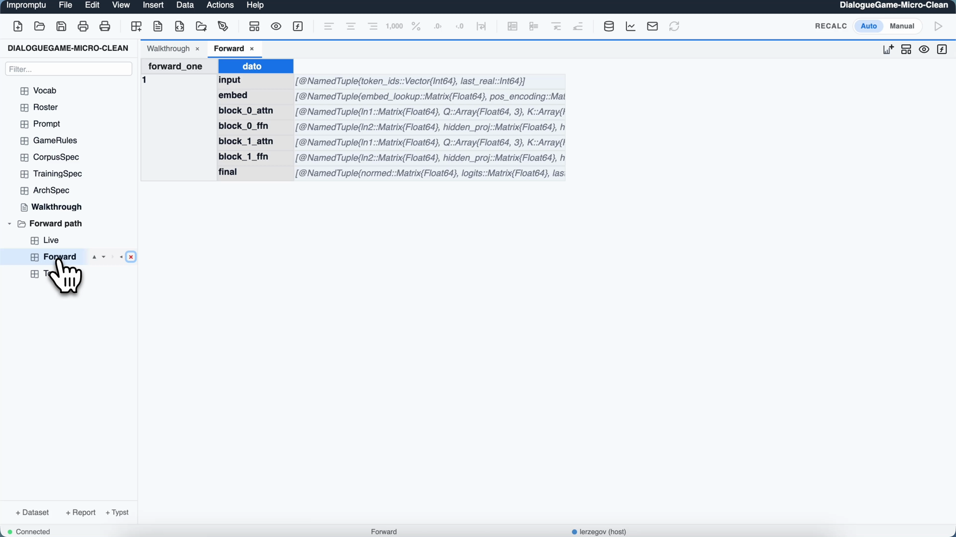
Forward dataset, the whole fast path: seven Object cells (input, embed, block_0_attn, block_0_ffn, block_1_attn, block_1_ffn, final), each holding a @NamedTuple whose field names and types are all the grid can show of it. block_0_attn carries ln1, Q, K, …; final carries normed and logits. The architecture is legible. Not one of its numbers is.3. Transparency mode, a second implementation in cells
A second script, materialise_detail_view, is labelled Materialise Detail View (Transparency Mode) in the Actions menu. It does two things, and the distinction between them matters.
It projects the weights out of Live.bundle into ordinary datasets: a copy of the numbers, laid out under named dimensions. And it writes a second forward pass, as a chain of ordinary formulas over those datasets, computing the same thing the seven compiled Object cells compute. The Objects are not unfolded. The same network is implemented twice, once compactly and once legibly, in one model. Thirty-two datasets come out of it, in two families.
Sixteen weight datasets. One per weight matrix, dimensioned by the same architecture dims the scaffold created:
| dataset | dimensions | cells |
|---|---|---|
Embeddings |
vocab × d_model | 1,792 |
W_q, W_k, W_v |
layer × d_model × head × d_head | 8,192 each |
W_o |
layer × head × d_head × d_model | 8,192 |
W_ff_up |
layer × d_model × d_ff | 32,768 |
W_ff_down |
layer × d_ff × d_model | 32,768 |
b_q, b_k, b_v, b_o, b_ff_up, b_ff_down |
(biases) | 1,152 total |
LN1, LN2 |
layer × d_model, gamma + beta |
256 each |
FinalNorm |
d_model, gamma + beta |
128 |
That is 101,888 cells in all, the trained model laid out flat. The ≈107,000 figure quoted in the main post is that number plus the 80 × 64 sinusoidal position table. The position table is computed, by the formula pos_encoding = llm_pos_encoding(80, 64), not learned, so the larger figure is a fair count of the network and not a fair count of the parameters. The distinction is spelled out because the point of the exercise is that the numbers are checkable.
Sixteen forward-pass datasets. The same computation the seven Objects did, now written out step by step: Input, EmbedSeq, then per layer a QKV, an AttnScores, a HeadOut, an FFNHidden and a Block_L, then FinalNormOut, Logits, NextToken and TopK. That is 319,916 cells. Block_0_AttnScores alone is 4 heads × 80 query positions × 80 key positions, twice (raw scores and post-softmax weights), which is 51,200 cells of attention pattern that can be scrolled through.
The cell chain is not quite self-contained. It leans on the compiled side in two places: Input tokenizes the prompt by calling llm_tokenize(Live.bundle, …), and TopK calls the bundle to turn token ids back into names. Tokenizing and naming stay compiled. Everything between them, every weight, every score and every intermediate vector, is a cell.
The script also switches auto-recalculation off when it finishes. That is a conservative default for a chain this size, and it is an ordinary model setting that can be turned back on. With recalculation on, this model keeps up: change the prompt, or clear a block of weights, and the dependent cells follow. The episode is shot that way.
One safeguard makes the arrangement more than decorative. Having built the new chain, the script recalculates it once and asserts parity: the cell-level NextToken must agree with what the seven-Object fast path produces, and with the bundle’s own forward pass. Two independent implementations, made to answer the same question, are checked against each other before either is handed over. That is what licenses reading the cells as the model rather than as an illustration of it. The check is performed at that moment; it is not an invariant that holds forever. Section 4 depends on that distinction.
4. Weights are just more datasets, so the ablation is a cell edit
W_o is the output projection that writes each attention head’s result back into the residual stream. It is a dataset with four dimensions: layer, head, d_head, d_model. Set layer = L0 and head = h3 in the grid’s dimension selectors, and what remains on screen is a 16 × 64 block of 1,024 cells, the slice of the weight matrix belonging to layer 0, head 3.
Select that block and clear it. That is a head ablation. It takes a range selection and a delete. In this engine there is no hook to attach, no forward function to patch and no configuration flag.
The formulas downstream of W_o are ordinary formulas, so the change propagates through both blocks the way any spreadsheet change propagates. With recalculation live it happens on the spot. In the episode, on the prompt
<BOS> Pietro chiama Paolo <SEP> Paolo chiama 4 <SEP>the model predicts 4 at probability 0.99933. That is the chain rule, copying the name just called. Zeroing L0·h3’s block flips the top prediction to 2 and collapses p(4) to 0.0005. Zeroing an inert layer-1 head instead leaves 4 at 0.999. Undo restores it.
The parity check from §3 is useful here because it stops holding. The edit lands on the projected weights, which the cell chain reads. It does not touch Live.bundle, which has no formula and is nobody’s dependency. After the delete the two implementations disagree: the cells compute an ablated network while the compact fast path still holds the intact one. That disagreement is the experiment. Parity established that the two agreed about the model as trained; breaking it in one named place is the intervention.
The same intervention can be run automatically. run_head_ablation_lean is an engine script that zeroes every head in turn, re-measures rule accuracy on the held-out split, and writes the results into a HeadAblation dataset. For L0·h3 it reports what the hand edit reports. The by-hand demonstration and the systematic probe are the same intervention carried out by different means, which is the reason to trust either.
Nobody built an ablation feature. The edit works because a weight has no special status in the model: it is a cell, on a dataset, with dimensions, like a revenue assumption.
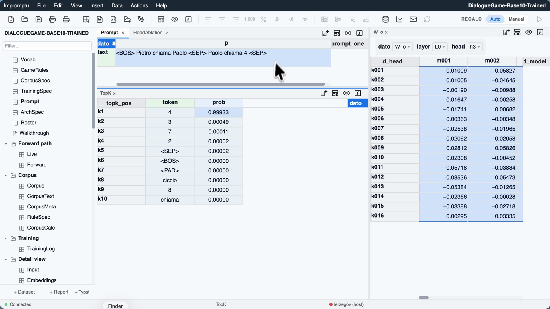
W_o open on the right, with its layer and head selectors set to L0 and h3 and the whole 1,024-cell block selected. The values are ordinary trained numbers: 0.01009, 0.05827, −0.00190. On the left, the prompt <BOS> Pietro chiama Paolo <SEP> Paolo chiama 4 <SEP>, and below it TopK showing the chain-rule copy, 4 at 0.99933.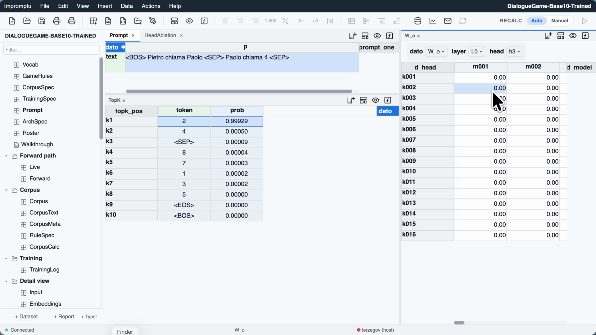
TopK now reads 2 at 0.99929, with 4 down to 0.00050. The prediction changed because a range of cells changed.5. The forward pass is a recalculation
In the cell-level implementation, a Transformer block is written as formulas, and running them is what produces the numbers. A block, in full, looks like this (the actual formula text of the Block_0 dataset, in the engine’s terse algebra mode):
ln1       = llm_layernorm(EmbedSeq.x, LN1.gamma[1, :], LN1.beta[1, :])
attn_out  = let
  HO = Block_0_HeadOut.out
  out = zeros(Float64, 80, 64)
  for h in 1:4
    out .+= HO[h, :, :] * W_o.W_o[1, h, :, :]
  end
  out .+ b_o.b_o[1, :]'
end
post_attn = EmbedSeq.x .+ attn_out
ln2       = llm_layernorm(post_attn, LN2.gamma[1, :], LN2.beta[1, :])
ffn_out   = Block_0_FFNHidden.act * W_ff_down.W_ff_down[1, :, :] .+ b_ff_down.b_ff_down[1, :]'
block_out = post_attn .+ ffn_out
Every line of the Transformer’s block equation is one array-level formula over named datasets. post_attn = EmbedSeq.x .+ attn_out is the residual connection: one addition. The loop over h is the four heads writing into the stream through their W_o slices, the same slices the ablation selects and zeroes.
The readout, the step the main post spends its Act 1 centrepiece on, is one cell. The ReadoutTerms dataset holds the two vectors, and Readout reduces them:
# ReadoutTerms — vocab × d_model
emb       = Embeddings.W_embed
resid     = FinalNormOut.normed[t011]
dot_term  = emb * resid

# Readout — vocab
logit  = ReadoutTerms.dot_term[d_model: sum]
cosine = ReadoutTerms.dot_term[d_model: sum] /
         (sqrt(ReadoutTerms.emb_sq[d_model: sum]) * sqrt(ReadoutTerms.resid_sq[d_model: sum]))
\text{logit}(t) = h \cdot e_t, the dot product of the residual with each token’s embedding, is dot_term[d_model: sum]: multiply elementwise across the d_model dimension, then sum along it. The whole unembedding, for the whole vocabulary at once, is that one line. The cosine on the line below is the same quantity divided by the two lengths. The two numbers the main post presents as the same fact seen twice are, here, two formulas sharing a subexpression.
This is why the model runs when something changes. Edit the prompt and the tokenizer cell recomputes, then the embedding, both blocks and the logits. Edit a weight and the same graph recomputes from that weight forward. Nothing calls an inference routine. On this side of the model the forward pass is the recalculation, in the ordinary spreadsheet sense, not so different from the mechanism that carries a changed growth assumption through a cash-flow statement. The compiled side is still there, one dataset away, computing the same prediction its own way. That is the reason for having both.
6. The other half of the machine, action scripts
Everything above was built by launching scripts from buttons, and the buttons need explaining, because they are the one part of this system a user cannot author.
Impromptu has two kinds of thing that make a model change.
Formulas are user content. A user writes them into a dataset; they are stored in the model file; the engine recomputes them whenever something they depend on changes. Readout.logit, Block_0.post_attn and the CorpusCalc lines the main post compares against are all formulas. If a formula is wrong, the user edits it.
Action scripts are engine code. An action is a named, parameterised Julia function, registered inside the engine at startup, that takes the model and mutates it. It is not stored in the model file, and there is no way to write or edit one from the interface: no action editor, no scripting cell. From the UI an action has exactly one affordance, which is to launch it. There are two places to do that from:
- the Actions menu, which lists every registered action grouped by category (the eight below all sit under “Language model”) and prompts for parameters; and
- an
action://link inside a report. A markdown report can carry[▶ Scaffold](action://scaffold_forward)or[▶ Corpus](action://generate_dialogue_corpus?rule_mode=basic), and clicking it fires that action with those parameters against the model the report belongs to.
The second is what the episode’s Walkthrough report is: a page of prose with seven buttons in it, in order (Scaffold, Corpus, Train, Glass box, Inspect, Ablate, Simulate), so that building the model from a clean slate is a readable sequence rather than a menu-diving exercise. A document about the model can operate the model, which is useful for teaching. It is still not an action editor: the report author chooses which registered action to link, and nothing else.
(A terminology collision to head off: the general engine note uses the word “actions” for the set of typed model-building operations the AI assistant reaches through the MCP channel, such as create dataset and set formulas. Those are a different thing, on a different seam. Everything in this section is about action scripts: registered Julia functions launched from the UI.)
Why the corpus is a script and not a formula
This distinction is the reason the main post is careful about where its training data comes from. It is also the easiest thing in the whole setup to get backwards, so it is stated here plainly.
The corpus is not generated by spreadsheet formulas. It is written by the generate_dialogue_corpus action, a Julia script that runs the game simulator n_rounds times and writes 800,000 token cells into a Corpus dataset (plus another 800,000 readable strings into CorpusText). It has to be a script for two reasons, both about the nature of a formula:
- A formula may not roll dice. Formulas are recomputed, and a formula calling
random()would produce a different corpus on every recalculation; the training data would move under the model. The action takes its seed fromCorpusSpec.seedand constructs its own generator, so the same model with the same seed yields a byte-identical corpus every time. Reproducibility is the reason the corpus is written down rather than derived. - The rule is procedural. A round is a loop with state: whoever was just called becomes the caller, players have per-player error probabilities, the round ends when a condition trips. That is a simulator, not an expression.
The rules of the game are also written as formulas, in a dataset called CorpusCalc, which reconstructs the corpus from ten lines and nothing else, replaying the same seeded draws through a formula-side function rather than a generator. This is what makes the episode’s ending possible. CorpusCalc is never used for training. It exists so there is something exact and readable to hold the trained weights up against, and it reproduces the first thousand training rounds string for string. Both statements are true at once, and they are about different objects: the corpus was written by a script, and the rules are ten formulas in a cell grid.
The one-way seam
There is one asymmetry in all this that took a while to notice, and I think it is the actual design principle. Action scripts write formulas. Formulas never write code.
scaffold_forward does more than create the Forward dataset: it generates the formula text for it, one attention line and one feed-forward line per layer, from ArchSpec.n_layers. materialise_detail_view generates the entire sixteen-dataset algebra chain the same way. What an action leaves behind is cells, dimensions and formulas: ordinary model content, saved in the model file, editable afterwards by hand. The script is a builder. Once it has run, the user is back in a spreadsheet, holding something that can be read and changed.
This is why the ablation works. If the glass box were rendered by a viewer written in engine code, zeroing a weight would need a feature. Because it is built out of ordinary model content, zeroing a weight needs nothing at all.
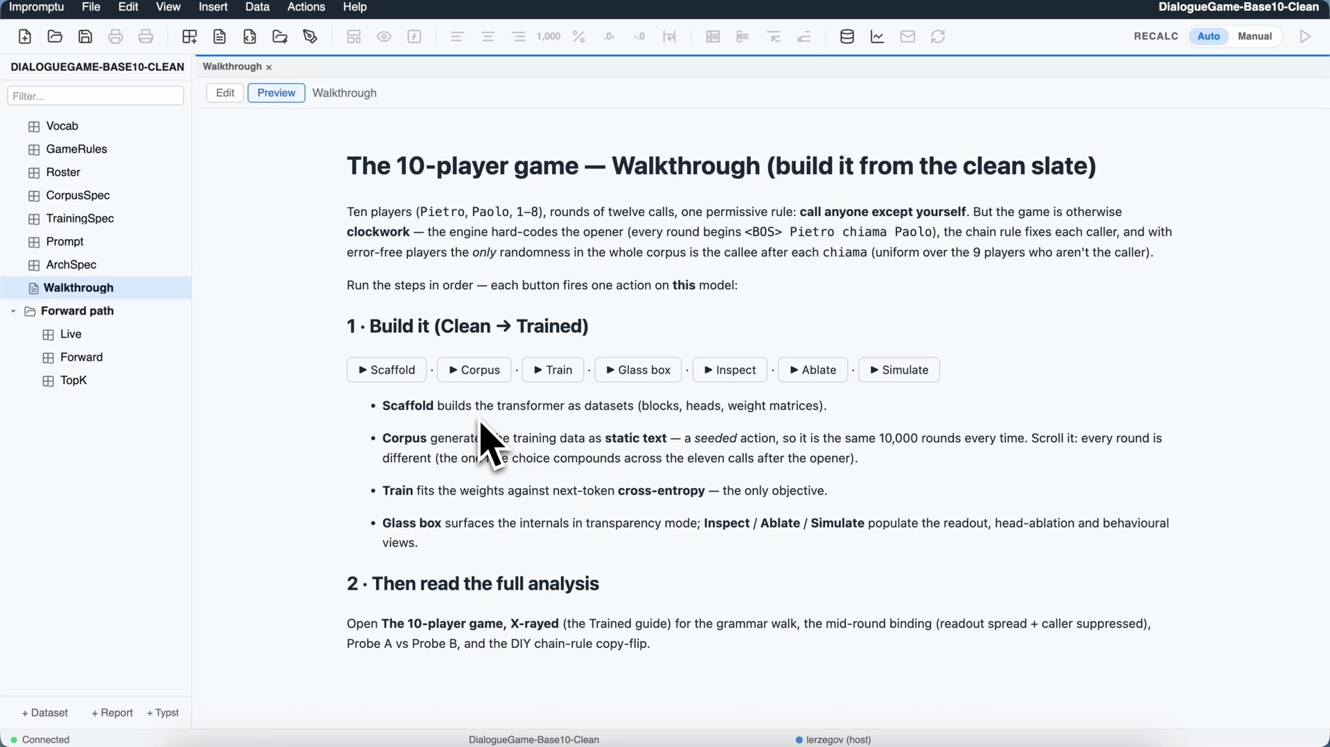
Walkthrough report, rendered inside the model. The row under “1 · Build it” is seven action:// links (Scaffold, Corpus, Train, Glass box, Inspect, Ablate, Simulate) rendered as buttons; pressing one runs that engine script on this model and refreshes the report. This is the second half of the machine as a reader meets it: prose, and things that can only be launched.7. The gain, the limit and the cost
The gain. Every claim in the main post is a claim about something selectable, which is what the whole series stands on. Act 1’s residual-stream climb from 0.08 to 8.15 is five successive reads off the same block chain. The 0.978 cosine is a cell. The loss floor at 0.514 is a row in TrainingLog. The head that carries the copy is a 1,024-cell block that can be deleted and undone. When a number appears in a post here, there is a coordinate behind it, and an intervention behind it: an input can be changed and what depends on it watched, which is a stronger form of evidence than a printout.
The limit. The second implementation does not supply answers. The main post’s real finding is negative: “call anyone except yourself” has no localisable implementation in the trained weights, and the largest single-head ablation still leaves the rule standing at 0.860. Full visibility into 101,888 numbers did not turn into an explanation. Transparency is a precondition for interpretability. It does not replace it. The glass box makes it possible to ask precisely, and the asking is still hard.
The cost. This scales to a hundred thousand parameters, not a hundred billion. The glass-box chain is 320,000 cells for a 2 × 4 × 64 model and an 80-token window. The attention scores alone grow with the square of the context, so the same construction on a longer context stops being comfortable well before it stops being possible, which is why the script’s own default is to switch live recalculation off and leave it to the user to turn on. This is a bench instrument for models small enough to see, and the series is built around models small enough to see because that is the regime where the instrument works.
Impromptu is my own research bench, a prototype I built to be able to open the hood on things like this, not a product you can download. The way to see the grids described here is the episode’s screen recordings, embedded in Clockwork and dice: the W_o block being selected and zeroed, and the prediction flipping, happen on camera.
Appendix A, what an action script looks like
Three excerpts of real engine source, chosen because they are short enough to read whole. This is engine code: it lives in the Julia codebase, ships with the engine, and is read-only from the interface.
A.1, the registry
Every action is one register_action! call. The definition names the action, labels it for the menu, declares its parameters, and points at the function that does the work. This is the whole contract (XModel/src/actions.jl; the field comments are mine, condensed from the docstring above it):
struct ActionDef
    name::String            # machine identifier, the `action://` target
    label::String           # display name in the Actions menu
    description::String     # help text shown in the UI
    category::String        # grouping label, e.g. "Language model"
    params::Vector{ActionParam}
    execute::Function       # (model::Model, params::Dict) -> ActionResult
end

"""Global action registry. Populated at module load time."""
const ACTION_REGISTRY = OrderedDict{String, ActionDef}()

function register_action!(def::ActionDef)
    ACTION_REGISTRY[def.name] = def
    def
end
Two lines of that carry the whole distinction this note is about. ACTION_REGISTRY is global and populated at module load time, so the set of actions is fixed by the running engine, not by the open model. And execute is a Function, a compiled Julia closure, which is why the model file can name an action but can never contain one.
An ActionResult reports what changed (success, a message, and the datasets touched) so the server can tell every connected browser which grids to refresh.
This is scaffold_forward’s registration, abridged (dialogue_game/forward_dataset.jl):
register_action!(ActionDef(
    "scaffold_forward",
    "Scaffold Forward Variant",
    "Builds (or rebuilds) the Forward variant on a clean DialogueGame base " *
    "(with ArchSpec). ...",              # … full help text elided
    "Language model",
    [
        ActionParam("n_layers",  :int,
            "Transformer block count (>=1). Empty → use current ArchSpec.", 0),
        ActionParam("n_heads",   :int,
            "Attention head count. Must divide embed_dim. Empty → use current.", 0),
        ActionParam("embed_dim", :int,
            "Residual stream width. Must be divisible by n_heads. Empty → use current.", 0),
        # … ffn_dim, seq_len, topk_n
    ],
    _execute_scaffold_forward
))
Those parameter declarations are what the Actions menu builds its dialog from, and what an action://scaffold_forward?n_layers=4 link would fill in.
A.2, the builder that writes formulas
The part of _execute_scaffold_forward that matters here is this helper, which generates the formula source for the Forward dataset from the layer count. It is engine code producing user-editable model content, the one-way seam from §6, in a dozen lines (the blank-line spacers it also emits are elided here):
function _dg_forward_formula_chain(n_layers::Int, seq_len::Int, topk_n::Int)::String
    lines = String[]
    push!(lines, "input = llm_input_pack(Live.bundle, Prompt.text, $seq_len)")
    push!(lines, "embed = llm_embed_pack(Live.bundle, input.token_ids)")
    prev_out = "embed.x"
    for L in 0:(n_layers - 1)
        push!(lines, "block_$(L)_attn = llm_block_attn_pack(Live.bundle, $(L+1), $prev_out)")
        push!(lines, "block_$(L)_ffn  = llm_block_ffn_pack(Live.bundle, $(L+1), block_$(L)_attn.post_attn)")
        prev_out = "block_$(L)_ffn.block_out"
    end
    push!(lines, "final = llm_final_pack(Live.bundle, $prev_out, input.last_real, $topk_n)")
    join(lines, "\n")
end
The caller then creates one Object cell per line and hands the string to the formula compiler:
forward_src = _dg_forward_formula_chain(n_layers, seq_len, topk_n)
success, errors = update_dataset_formulas!(model.datasets["Forward"], model, forward_src)
After that call the action’s job is done and the network is a spreadsheet.
A.3, the same rule twice
This is the smallest comparison in the whole system: “call anyone except yourself” as engine code, in the simulator that writes the corpus (dialogue_game/simulator.jl):
function caller_callable_set(r::Roster, caller::AbstractString)
    cs = r.callable_sets
    cur = String(caller)
    if cs !== nothing && haskey(cs, cur)
        return cs[cur]                      # a restricted rule variant
    end
    return [p for p in r.players if p != cur]   # the default: anyone but me
end
And this is the same rule as a formula, in the CorpusCalc dataset the main post compares the trained weights against. There is no list to filter, only a draw from 1…9 that steps over the caller’s own seat:
callee_pos[call:rest] = Int(text_to_value(draw)
                       + (text_to_value(draw) >= text_to_value(caller_pos)))
The rule appears once on each side of the seam: as a filter in a compiled function, and as an arithmetic expression in a cell. The model was trained on the output of the first and measured against the second, and the two agree exactly: zero self-calls in the 12,000 calls checked, those being the 1,000 rounds of twelve calls that CorpusCalc reproduces byte for byte against the generator’s own output.
Appendix B, the eight scripts the episode uses
All eight are registered under the category Language model and live in XModel/src/dialogue_game/. They are read-only from the interface and launchable from the Actions menu or an action:// link.
| Action | Source file | What it does |
|---|---|---|
scaffold_forward |
forward_dataset.jl |
Reads ArchSpec, creates the architecture dimensions, initialises the network into the Live.bundle Object cell, and generates the seven-cell Forward formula chain. |
generate_dialogue_corpus |
actions.jl |
Runs the seeded game simulator n_rounds times and writes the token corpus (Corpus) and its readable twin (CorpusText); persists the resolved rule to RuleSpec so the trainer scores the same rule. |
train_dialogue_model |
training.jl |
Runs the trainer as a subprocess against Corpus using the settings in TrainingSpec, writes one row per logged epoch into TrainingLog, and loads the trained weights back into the model. |
materialise_detail_view |
materialise_detail.jl |
Transparency mode: projects Live.bundle’s weights into sixteen datasets, writes a parallel sixteen-dataset formula forward pass over them, asserts parity against the compiled fast path, and leaves live recalculation off by default. |
refresh_inspection_views |
inspect_views.jl |
Probe A. Runs one forward pass on a probe prompt and builds HeadCallerAttn, how much each head attends to the caller. Correlational. |
run_head_ablation_lean |
ablation_lean.jl |
Probe B. Zero-ablates each head in turn and re-measures rule accuracy on the validation split, writing HeadAblation. Causal: the automated form of the by-hand W_o edit. |
concept_trajectory |
concept_trajectory.jl |
Builds the residual-stream trajectory geometry as live formulas over the detail datasets, so the plotted plane moves when the prompt or a weight is edited. |
simulate_game_run_fast |
simulate.jl |
Greedy-decodes a whole game from a seed prompt against the trained network, one BLAS call per step rather than a full model recalculation, and logs each step’s top-k. |
The action://name?param=value → function mapping is the registry in XModel/src/actions.jl; the report-side button seam is the action:// link handler in the browser client.
Glossary
Terms specific to this note. The language-model vocabulary (token, logit, softmax, ablation, cross-entropy) is in the main post’s glossary.
Dataset. A named, multidimensional table in an Impromptu model. Its dimensions are named (layer, head, d_model), its columns are named arrays, and formulas are written over those names rather than over cell addresses. W_o is a dataset with four dimensions.
Array-level formula. A formula assigned to a whole array rather than to one cell. post_attn = EmbedSeq.x .+ attn_out computes 80 × 64 values in one expression, which is why a Transformer block fits in six lines.
Object cell. Impromptu’s fifth cell type, alongside number, text, date and datetime. It can hold any Julia value; here, the entire network as one structured value in Live.bundle. Always formula-computed, except where, as with Live.bundle, the absence of a formula is deliberate so that a written value survives recalculation.
Transparency mode. The state a model is in after materialise_detail_view has run: the weights copied out of the Object cell into ordinary datasets, and a second forward pass written as formulas over them, alongside the compiled one. Live recalculation is left off by default and can be turned back on.
Recalculation. Impromptu’s dependency-driven recompute, the same mechanism that propagates a changed assumption through a financial model. On the cell-level implementation of a language model, running it is the forward pass.
Action script. A named, parameterised Julia function registered in the engine’s action registry, launched from the Actions menu or an action:// link in a report. Engine code rather than model content: it is not stored in the model file and cannot be authored or edited from the interface.
action:// link. A markdown link inside a report that fires a registered action against the model the report belongs to, for example [▶ Corpus](action://generate_dialogue_corpus?rule_mode=basic). It is how the Walkthrough report turns a build sequence into a page of buttons.
Parity assertion. The check materialise_detail_view runs after building the cell-level chain: its prediction must match the compiled fast path’s and the bundle’s. It is what licenses reading the cells as the model. It is a check made at that moment, not a standing invariant. Editing a weight breaks it on purpose, and that is the ablation.
Further reading on this blog
The machinery, on models too big to see. Three earlier notes explain the Transformer itself, without a bench or a video. They are the reference for the vocabulary used above, and they run in order:
- Transformers and QKV Attention: A Primer. How information moves between words: queries, keys, values, the residual stream, and why attention is the only channel through which tokens exchange information.
- Embeddings and the Maps We Draw of Them. Where the vectors come from, why hand-wiring meaning fails, and how to look at a high-dimensional space without being misled by the picture.
- The Final Step: The Language Model as a Relentless Seeker of the Best Next Word. The readout as a similarity search, and what falls out of one dot product. §5 above is that final step, with the dot product as a cell formula.
The experiment. Clockwork and dice, the post this note accompanies: a language model trained on a world whose rules we wrote ourselves, and what happened when we went looking for the rule in the weights.
The engine. Impromptu under the hood, the general tour: two tiers, Julia and Elm, the formula language, typed cells, and the assistant at the bench.
This is the technical companion to Clockwork and dice, episode 1 of the ABC of language models.