Who is still at the table, part I: a small model keeps the score by heart
Episode 3 of the ABC of language models, and Part I of a two-part story, “Chi resta al tavolo” (who is still at the table). Each note in the series is built around a model small enough to take apart on the bench. Episode 1, Clockwork and dice, taught a tiny Transformer a calling game whose rules we wrote ourselves. Episode 2, Lying dice, put one unreliable player at the table and found the error rate at which the model’s best guess becomes the mistake. This episode lets mistakes remove players from the game, and asks whether a small model can keep track of who is left. Part II, “Il segnapunti” (the scorekeeper), is in production: it moves that knowledge out of the model. The companion video is embedded below; the post is readable on its own. Everything is built and taken apart inside Impromptu, a modeling engine I built from scratch: my own research bench, not a product you can download. New ideas are explained where they first matter, in boxes like the one below. The detailed measurements are in the appendices; Episode 1’s glossary still applies, and this post adds its own entries at the foot.
TL;DR
The calling game of the first two episodes gets one new rule: whoever errs leaves the table. A mistake is calling a player who is already out, or saying one of four words that are not names: boh, nonno, ciao, cavolo. No player ever calls their own name. After the opening call, every call is a mistake one time in four. The game runs eight rounds, one elimination per round, until two players are left and are named the winners. The transcript records each elimination once, as a line like 5 perde (“5 loses”), and never again. Nowhere does it say who is still seated.
I trained a small language model on 20,000 transcripts of this game and asked it three practical questions. Does it know who opens each round? Does it avoid calling players who are out, as much as the real players do? Can it name the two winners at the end?
The two-layer model answers all three. Over 10,000 new games it names the right opener 1.000 of the time in rounds 1 to 7 and 0.999 in round 8, and both winners in 9,997 games. Its one imperfection is a small leak: it keeps a little more probability on players who are already out. By the last round the game’s own odds (the rules the transcripts were generated from) put 0.159 of a caller’s probability on eliminated players, because in this game players do make that mistake; the model puts 0.237. A one-layer model cannot do the job: by round 8 it names the right opener in 0.585 of games and both winners in about half (0.519). A four-layer model, twice as wide, leaks much less: 0.169 in round 8.
Then I opened the model to see how it keeps the score. The result was not what the well-known Othello experiment would predict. Information about who is out can be read off the model’s internal numbers, but editing that information barely changes what the model does. What the model relies on is a two-step look-up. One attention head marks every X perde line with the name of the player who lost, and two heads of the next layer, which have divided the players between them, look back at those lines at every decision. Switch off the marking head and the model loses the table. The model does not carry a running scoreboard. It recomputes who is seated from the record of the game, every time it needs to know.
That has a cost. Each decision means re-reading a transcript that only gets longer, and a model can follow only the rules it was trained on. Part II takes up both.
The game: whoever errs leaves the table
The world is still Pietro chiama Paolo, the calling game of the first two episodes. Ten players: Pietro, Paolo, and 1 through 8. Whoever is called speaks next and calls somebody else. The one choice in the game is whom to call.
In episode 2 a mistake ended the round and everybody stayed. Here a mistake costs the player their seat. There are two kinds of mistake: calling somebody who has already left, or saying one of four words that are not names, boh (“dunno”), nonno (“grandpa”), ciao and cavolo (“cabbage”, or “darn”). After the opening call, every call is a mistake one time in four, for every player (p = 0.75 is the chance of a correct call), and the mistake is spread evenly over the four words and the players already out. A correct call goes to one of the other seated players, all equally likely; no player ever calls their own name. The transcripts come from a game engine that plays by these rules: it always knows who is seated, and at each call it draws a correct callee three times in four and a mistake once in four, on purpose. Every round of the corpus therefore ends with exactly one mistake, the one that eliminates its caller. The first three rounds of a game the model never saw in training:
<BOS> Pietro chiama Paolo <SEP> Paolo chiama 2 <SEP> 2 chiama Paolo <SEP> Paolo chiama nonno <SEP> Paolo perde <SEP>
Pietro chiama 1 <SEP> 1 chiama 2 <SEP> 2 chiama 7 <SEP> 7 chiama 6 <SEP> 6 chiama nonno <SEP> 6 perde <SEP>
Pietro chiama 1 <SEP> 1 chiama boh <SEP> 1 perde <SEP> …
Paolo, then 6, then 1 say a word and leave. In the fourth round 8 calls 1, who left in the third round. That is the other mistake, and 8 is out too. After eight rounds two players remain, and the transcript closes on vincono A e B <EOS> (“A and B win”); this game closes on vincono 2 e 7. The video plays this game out (from 1:02).
The three episodes differ in one thing: who makes mistakes, and what a mistake does. In every case the mistakes are drawn by the game engine at a rate we set, so the rate is a dial and the correct answer is known in advance.
| episode | who makes mistakes | the mistake | what it does | the dial |
|---|---|---|---|---|
| 1, Clockwork and dice | nobody | none | none: every call is correct | |
| 2, Lying dice | one player, 5, a systematic offender |
he calls himself | ends the round; everybody stays | his rate, from 0 to 0.20 over seven models |
| 3 and 4, this story | every player alike | a call to a player already out, or one of four words that are not names | eliminates the caller | one rate for everybody, here 0.25 |
In episodes 3 and 4 nobody lies. Every player is honest and occasionally slips: they forget that a player has already left, or they blurt out a word instead of a name. The four words are there for round 1, when nobody is out yet: a round must be able to end on a mistake from the very first call.
Two details matter for what follows.
Each round is opened by the first two players still seated, in the order of the roster (Pietro, Paolo, 1, 2, …, 8). While Pietro and Paolo are both in, every round opens Pietro chiama Paolo. Once one of them is out, the opener moves down the roster. So knowing who opens a round means knowing who is still in.
And the transcript never states the table. It says Paolo perde once, at the moment it happens. A hundred words later, in round 6, a player who wants to know whether Paolo can be called has to remember that line or go and find it. This is the kind of uncertainty episode 2 promised at its close, and it is not really uncertainty: who is seated is a fact, fully determined by what has already happened.
The state is what you need to know right now to play correctly: here, who is still seated. The transcript is a record of events; the state is never written in it and must be derived. A ledger is the familiar case. The journal lists the entries; the balance is what you need to make a decision, and either someone keeps a running balance or someone adds up the journal when asked. Whether the model does the first or the second is the question of this episode.
The world’s odds
Every measurement in this post compares the model with the odds the transcripts were drawn from, so it is worth working them out once.
Take a free choice: any call after the opening one of a round. In round k (k = 1 in the first round) there are m = k - 1 players already out. The engine sorts what the caller can say into two kinds:
- legal names: the 9 - m other players still seated. Together they get p = 0.75, shared equally, so 0.75/(9-m) each.
- mistakes: the four words and the m players already out, 4 + m in all. Together they get 1 - p = 0.25, shared equally, so 0.25/(4+m) each.
Each elimination moves one name from the first kind to the second, so the legal names get fewer and richer, the mistakes more numerous and poorer:
| round k | legal names | each gets | mistakes | each gets | on players already out | on the four words |
|---|---|---|---|---|---|---|
| 1 | 9 | 0.08333 | 4 | 0.06250 | 0.00000 | 0.25000 |
| 2 | 8 | 0.09375 | 5 | 0.05000 | 0.05000 | 0.20000 |
| 3 | 7 | 0.10714 | 6 | 0.04167 | 0.08333 | 0.16667 |
| 4 | 6 | 0.12500 | 7 | 0.03571 | 0.10714 | 0.14286 |
| 5 | 5 | 0.15000 | 8 | 0.03125 | 0.12500 | 0.12500 |
| 6 | 4 | 0.18750 | 9 | 0.02778 | 0.13889 | 0.11111 |
| 7 | 3 | 0.25000 | 10 | 0.02500 | 0.15000 | 0.10000 |
| 8 | 2 | 0.37500 | 11 | 0.02273 | 0.15909 | 0.09091 |
The column “on players already out” is the share this post measures: 0.25\,m/(4+m), the probability summed over the players who are out. The mistakes always share the same 0.25, and as the table empties more of it falls on players who are out: 0.050 in round 2, and in round 8 seven of the eleven mistakes, 0.25 \times 7/11 = 0.159, the world’s figure in the TL;DR. The four words take the rest of the 0.25, 1/(4+m), from 0.250 in round 1 to 0.091 in round 8. The video builds the table step by step (from 3:42).
I checked the table on the corpus itself, about 80,000 free choices per round over the 20,000 training games: the error rate reads between 0.250 and 0.252 in every round, and the share on players already out 0.1598 in round 8 against the formula’s 0.1591.
No mistake is ever the likeliest name
Episode 2 found a threshold: the chance of a correct call below which the single most likely word is a mistake. The same comparison applies here, round by round. A single mistake is likelier than a single legal name when
\frac{1-p}{4+m} \;>\; \frac{p}{9-m} \quad\Longleftrightarrow\quad p \;<\; p^{*}(m) = \frac{9-m}{13}.
In round 1 the threshold is p^* = 0.692, and each elimination lowers it by 1/13, down to 0.154 in round 8. The game is played at p = 0.75, above the threshold from the very first call. In round 1 that is 0.083 for each legal name against 0.063 for each word; in round 8, 0.375 against 0.023. So in every round the single most likely next name is one the rules allow, and the world was built that way.
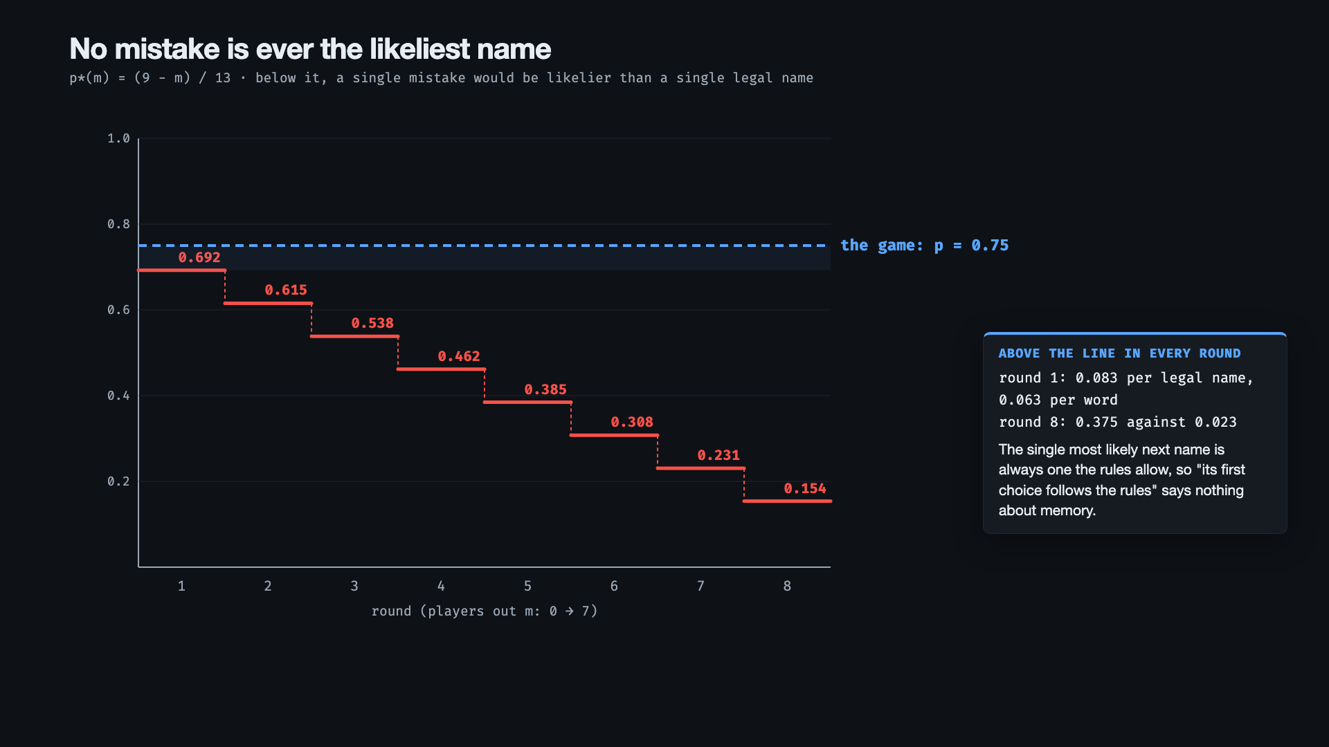
That has a consequence for how a model is graded. A model that has learnt the world’s odds always has a legal name as its first choice, whether or not it remembers who left. “Its first choice follows the rules” is therefore passed in every round by any model that has the odds roughly right, and says nothing about memory. The measurements below grade the probability the model spreads over the names instead, against the world it was trained on.
What keeping the table means, and how it is measured
A model that keeps the table perfectly is not a model that never calls an eliminated player. The real players do that, as part of the one time in four they slip, and a faithful model reproduces it. A credit model is judged the same way: a well-calibrated default model does not predict zero defaults, it predicts the rate that actually occurs. From here on, “the world” means those odds: the probabilities the engine draws each call from. So each measure compares the model’s probabilities with the world’s.
At every free choice the model gives a probability to each word it could say next. The mass on a set of names is the sum of those probabilities over the set: for example, the total probability the model puts on the players who are out. It is compared with the world’s mass on the same set, from the odds table.
At every free choice three masses are read, and they answer different questions:
- on the caller: 0 in the world, since no player ever calls their own name. Any mass here is a model error, and avoiding it needs no memory: the caller’s name is written one word back (
X chiama). - on the players out: the memory readout. To put the right share here the model must know who has left, including players who left six rounds ago.
- on the four words: noise, with no memory in it. Any call can be the one that ends the round, and no word is likelier than another.
Two more questions have exactly one right answer, so they are tests with no dice in them:
- Who opens the round? At the start of each round the model must name the first two seated players. It has one weakness, found while planning: the opener of round r is the previous opener unless the previous loser was one of them, so a model can get it right by looking back one round. It tests the latest update, not the whole table.
- Who won? At the end the model must write both winners’ names. That needs the whole history.
The models, and how they were trained
The model on camera is the same size as in episodes 1 and 2: a Transformer with two layers (L = 2), four attention heads in each (h = 4), and d_{\text{model}} = 64 numbers per position, the width of the residual stream. In the notation of the QKV primer, each head works in d_k = d_{\text{model}}/h = 16 dimensions, and each layer’s MLP in d_{\text{ff}} = 256. Beside it are two others, trained on the identical transcripts, so that the comparison is about the network alone: a one-layer model of the same width, and a four-layer model twice as wide:
| model | L | h | d_{\text{model}} | d_k = d_{\text{model}}/h | d_{\text{ff}} |
|---|---|---|---|---|---|
| one layer | 1 | 4 | 64 | 16 | 256 |
| two layers (on camera) | 2 | 4 | 64 | 16 | 256 |
| four layers | 4 | 4 | 128 | 32 | 512 |
A layer is one stage of processing. In each layer, every position can look back at every earlier position of the transcript (that is attention, done by several heads in parallel, each looking for something different) and then transform what it found. A second layer can look back at the results of the first. So depth decides how many steps a lookup can have when each step depends on the one before. Width decides how much each position can carry. Episodes 1 and 2 needed only two layers: the rule there depended on who was speaking, which is written one word back.
The training material: 20,000 games, 189 words each on average, at most 318. The model reads each game and, at every position, is scored on how much probability it gave to the word that actually came next. That score, the loss, has a floor. Some of the words are dice (whom to call is a free choice), and no model can predict dice better than their odds. Episode 1 introduced the floor; here it is computed from the world’s odds on the validation games at 0.3814 nats per word. A model at the floor has learned everything the transcripts contain except the dice.
Training adjusts the weights in small steps, each one in the direction that lowers the loss. The learning rate is the size of the step. Too small and training crawls; larger and it travels faster. Here the step is 1e-3, about three times the 3e-4 of episode 2. On the two-layer model the loss on the validation games fell from 2.22 after the first pass over the data to 0.587 after 16 passes and 0.401 after 50.
A large step has a known side effect near the bottom. A ball rolled fast into a bowl overshoots and swings back and forth before it settles. The loss does the same. On its passes 57 to 59 the two-layer model read 0.3906, 0.4055 and 0.3903: it was still swinging when the main phase ended. Its measurements at such a moment would describe the swing, not the model.
The anneal is a short last phase of training at a much smaller step: here five passes at one tenth of the learning rate (1e-4), starting from the weights the main phase ended with. It teaches the model nothing new; it lets it settle at the bottom of the bowl. Anyone who has used iterative calculation for a circular model in a spreadsheet knows the same move: big corrections to get close, small ones to land. In this episode every model was annealed before it was measured, so that two models are compared at rest, never mid-swing.
The two-layer model went from 0.3869 at the end of the main phase to 0.3849 after the anneal, and the five annealed passes agree to within 0.0003. Every model had the same budget: 60 passes at 1e-3, then the 5-pass anneal at 1e-4.
After the anneal, on the 2,000 validation games:
| model | passes over the data | distance from the floor, nats per word |
|---|---|---|
| one layer | 60 + 5 | 0.079 |
| two layers (on camera) | 60 + 5 | 0.0035 |
| four layers, twice as wide | 60 + 5 | 0.0013 |
The two-layer and four-layer models finish within 0.004 of the floor. The one-layer model stops more than twenty times further from it than the two-layer one.
Does it keep the table?
Every number in this section comes from 10,000 new games that none of the models saw in training (in the video from 5:43).
Who opens, and who wins
The two-layer model names the right opener 1.000 of the time in rounds 1 to 7 (one miss in 10,000 openers, in round 6) and 0.999 in round 8. At the end of the game it names both winners in 9,997 games out of 10,000. The four-layer model misses one opener in 10,000, in round 8, and names both winners in all 10,000 games.
Where the probability goes
The two easy readouts first. On the caller the two-layer model puts at most 0.0013 in any round, where the world puts 0. On the four words it follows the world closely: 0.241 against 0.250 in round 1, 0.099 against 0.091 in round 8.
The mass on players who are out, at the free choices of each round, against the world’s own share:
| round | 1 | 2 | 3 | 4 | 5 | 6 | 7 | 8 |
|---|---|---|---|---|---|---|---|---|
| players out | 0 | 1 | 2 | 3 | 4 | 5 | 6 | 7 |
| the world | 0 | 0.050 | 0.083 | 0.107 | 0.125 | 0.139 | 0.150 | 0.159 |
| two layers | 0 | 0.048 | 0.091 | 0.127 | 0.157 | 0.186 | 0.204 | 0.237 |
| four layers | 0 | 0.051 | 0.086 | 0.110 | 0.130 | 0.146 | 0.152 | 0.169 |
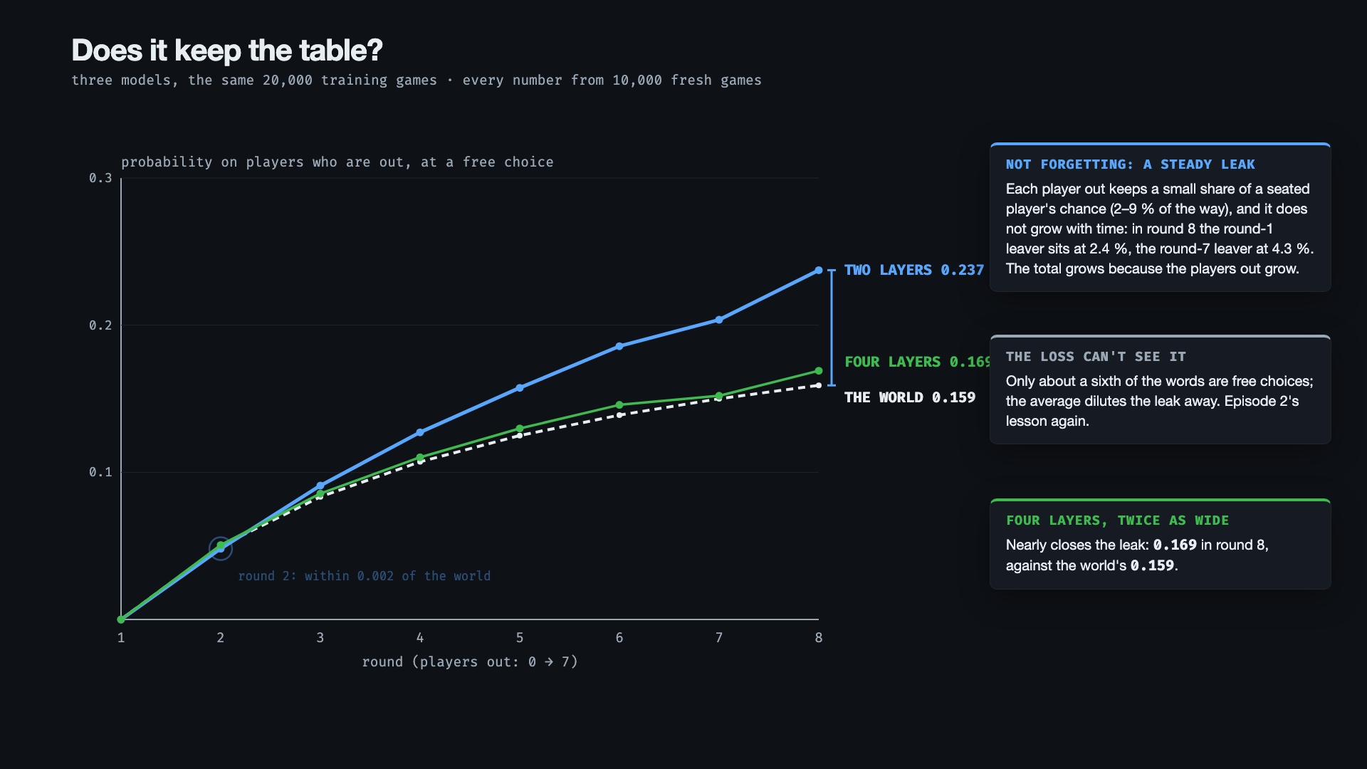
In round 2 the two-layer model is within 0.002 of the world. From round 3 it puts more on the eliminated players than the world does, and the gap widens as the table empties: by round 8 it is 0.237 against 0.159.
The excess has a simple shape. Each eliminated player keeps a small share of the probability a seated player would get: between 2 % and 9 % of the way from “out” to “in”, smaller in the later rounds (Appendix A). That share does not grow with time. In round 8 the player who left in round 1 sits at 2.4 % of the way, the one who left in round 7 at 4.3 %: if anything, the most recent elimination is the one held less firmly. So the model is not forgetting. It has a steady leak per player, and the leak adds up because the number of eliminated players grows by one each round.
Why a model close to the loss floor still leaks is episode 2’s lesson again. The loss is an average over every word, and only about a sixth of the words are free choices; the rest are scaffolding the model predicts almost perfectly. In round 8 the model’s excess over the world is 0.055 nats per free choice (Appendix A), which the average dilutes to a number the floor test cannot see. Training stops pushing on an error it barely pays for.
Why one layer fails and four leak less
The one-layer model is not on the floor, and it does not keep the table. Over 10,000 new games it names the right opener in every game of rounds 1 and 2, then 0.944 in round 3 and 0.585 in round 8; it names both winners in 5,187 games; in round 8 it puts 0.430 on eliminated players, where the world puts 0.159.
I did not dissect the one-layer model; in this story it marks the minimum: below a certain size, the model cannot keep the table. The structure suggests why. To know who opens round 6, the model has to find the lines where players left and then work out who that leaves at the front of the roster, a look-up whose second step depends on the first. A single layer gets one look back. Published work on small Transformers finds that copying information from earlier in the context, in the general case, appears only when two layers are stacked (Olsson et al., 2022, In-context learning and induction heads). That is a reading of the structure, not a measurement on this model.
The four-layer model leaks less than the two-layer one in every round from round 3 on, and by round 8 it is close to the world: 0.169 against 0.159, where two layers put 0.237. Each eliminated player keeps about 1 % of the way from “out” to “in” or less, with no trace of the two-layer model’s recency pattern (Appendix A). It is both deeper and wider, so this comparison says that more capacity reduces the leak, not which of the two does it.
How does it remember? Opening the box
The obvious guess comes from a well-known experiment, known as Othello-GPT (in the video from 8:18).
The game. Othello is played by two players, black and white, on a board of 8 × 8 = 64 squares. It starts with four discs in the centre. A move puts a disc of your colour on an empty square so that, in a straight line in any of the eight directions, it brackets one or more of your opponent’s discs between itself and a disc of yours; every bracketed disc flips to your colour. A move that flips nothing is not allowed, and a player with no allowed move passes. The game ends when neither player can move, after at most 60 moves, and whoever has more discs wins.
The transcript. A game is written down as the list of squares played, columns a–h, rows 1–8:
f5 d6 c3 d3 c4 …The board is never written: only the moves.
The experiment. In 2023, Li and colleagues generated millions of games in which each move was drawn at random among the allowed ones, and trained a language model (eight layers, d_{\text{model}} = 512) only to predict the next move (Emergent world representations, ICLR 2023). To do that well the model must know the current board, because which moves are allowed depends on it. They then did three things. They checked that the model’s next moves were almost always allowed ones. They found the board inside the model: a small classifier, a probe, could read each square (empty, black or white) off the model’s internal numbers, and later work showed that even a straight-line classifier can, once the squares are labelled as the current player’s or the opponent’s (Nanda, 2023). And they edited those numbers to flip a square, and the model’s predictions changed to the moves that would be allowed on the edited board. The board was not only readable; the model was using it. Kenneth Li, the paper’s first author, tells the story for a general audience in Do Large Language Models learn world models or just surface statistics? (The Gradient, 2023).
Their transcript and ours.
| Othello-GPT | this episode | |
|---|---|---|
| a word of the transcript | a square played | a name, a word that is not a name, chiama, or the line X perde |
| the state never written | 64 squares: empty, black or white | 10 players: in or out |
| the rules applied to the state | the allowed moves depend on the whole board | the legal names are the seated players other than the caller; the opener is the first two seated |
| the free choice | a random allowed move | a legal name three times in four, a mistake once in four |
| can the state be looked up? | partly: a square played once stays occupied, but its colour depends on every later flip, so it has to be computed | yes: each elimination is written once, as X perde, and nothing ever changes it back |
Our game is the same experiment at spreadsheet scale: ten players, in or out, instead of 64 squares, and two lines of rules instead of Othello’s. The last row of the table is the difference that matters. In Othello a model has to keep a board, because the colours can only be worked out by replaying every flip. In our game a model could keep a board too, or it could look the eliminations up whenever it needs them.
I used three instruments, all of them built as cells and formulas in the model, so that each can be inspected on the bench (Appendix B); the video uses them live (from 9:36).
As the model reads a transcript it keeps, for every word read so far, a list of 64 numbers: the residual stream. At the start the list only says which word this is and where it stands; each layer then adds what its heads and its MLP computed. The list at a word is what the model knows after reading up to there.
A probe asks whether that list contains the table. It is a logistic regression of the kind used in credit scoring, run once for each of the ten players: the explanatory variables are the 64 numbers, the dependent variable is 1 if player j is already out at that point of the game and 0 if they are seated. Ten regressions, ten scorecards, each with its own 64 coefficients. If a probe scores well, the information is present.
The 64 coefficients of probe j also form an arrow in the space of the 64 numbers, the probe direction for player j: the shortest way from “seated” to “out”, the direction in which that probe’s score rises fastest. In credit-scoring terms, the quickest way to raise one applicant’s score is to raise each feature in proportion to its coefficient; that proportional move is the direction.
A push (an intervention) edits the 64 numbers along that arrow while the model runs, to write “player j is out” into it. The size of the edit is its dose: a push of dose 8 raises the probe’s own score, its logit, by exactly 8. If the model uses what the probe reads to decide who opens the round, the opener changes. A push in a random direction of the same length is the control.
An ablation switches one attention head off. Its cost here is the drop in opener accuracy when the head is off. Episode 2 used it to find the head that reads who is speaking.
Reading. The information is there, and it sharpens with depth. The probes were fitted on 200 games and tested on 200 others. Early in a game almost every player is seated, so a probe that always answers “seated” would already score well on plain accuracy (0.638 here). The score that matters is the balanced accuracy: the average of two hit rates, how often the probe says “out” for a player who is out, and how often it says “seated” for one who is seated. A probe that always answers “seated” scores 0.5 on it. The balanced accuracy is 0.673 on the input alone (the word and its position, before any processing: late positions in a game have more players out), 0.759 after the first layer and 0.906 after the second.
Pushing. Writing “player j is out” along the probe direction barely moves the model. On the round-8 opener of the game above, where the seated players are 2, 5 and 7 and the answer is 2, a push of dose 8 on player 2 after the first layer takes the probe’s reading for 2 to 1.00 (“out”), and the model still says 2, at 1.000. I tried many variants: four ways of finding the direction, every layer separately and all at once, the edit at the opener alone or along the whole transcript, and doses up to 32, each beside its random control. After the second layer the push changes the opener in 0.004 of the cases, against 0.003 for the random push. After the first layer, at the largest dose only, it changes it in about a fifth of the cases (0.194 against 0.055 for random), through the second layer’s MLP at the point of decision and not through the heads that look back over the game. Othello’s test does not pass here. The information the probe reads is real, and it is not what the model uses to decide.
Following the attention. A head’s attention is where it looks: from the current word, a row of weights over the earlier words that sums to 1. What a head writes is a separate matter, set by its own output weights: looking at a word can raise, lower or leave unchanged the probability of any name. Both can be read in cells, and the model’s working heads are best named by what they do.
- The stamp head (first layer). At every word it looks at the word just before. At each
perdethat word is the name of the player who lost, and the head looks at it 0.968 of the time. So after the first layer, the position ofperdecarries who lost, not only that someone did. - Two look-up heads (second layer). At every decision they look back at the earlier
perdelines: from the openers, the main one puts 0.44 of its attention there on average and the second one 0.26. What they write is “not X”: seeing “Paolo perde”, the main look-up head lowers Paolo.
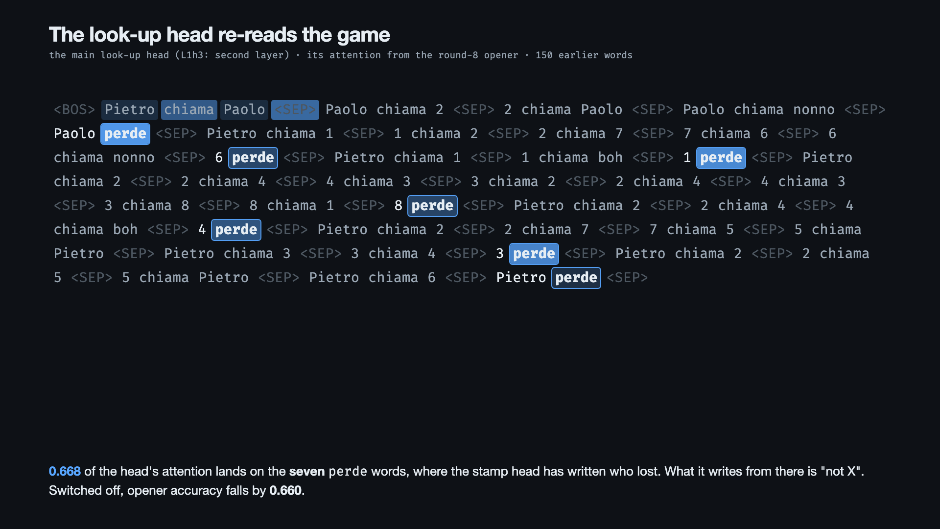
perde words carry 0.668 of it.
The two look-up heads have divided the roster between them. For each name, the main head lowers it strongly when it sees that name’s perde line (Paolo by 29.0, 7 by 16.3, 3 by 12.6, 5 by 12.5, 1 by 7.5, in units of the logit, the score that the final softmax turns into probabilities), but it writes almost nothing on Pietro and on 8. The second head’s two strong entries are exactly those two names (Pietro −8.7, 8 −7.5). Like two clerks who share a client list, each strikes off its own names, and between them every player is covered. Nobody assigned the split; it came out of training.
Switching heads off confirms the roles. Over 2,400 openers of 300 games, switching off the stamp head costs 0.797 of opener accuracy, the main look-up head 0.660, the second look-up head 0.338; the other heads cost between 0 and 0.125. With the stamp head off, the curve of the previous section breaks: opener accuracy falls to 0.16 in round 2 and 0.02 in round 8, and the mass on players out in round 8 rises from 0.236 to 0.670 (500 games). No stamp, nothing to look up.
So the model keeps no running balance. At every decision it adds up the journal: it goes back to the lines where players left and works out from them who is still seated. The “is out” signal that the probe reads is present, sharper layer after layer, and is not on the path to the answer. What the model uses is the record, marked by one head and re-read by two others.
Why Othello-GPT could be pushed and this model cannot. Othello-GPT passed both halves of the test: its board could be read and, once edited, it changed the moves. This model passes the first half, less sharply, and fails the second. Three differences account for that, and the measurements here cannot separate them.
- Size. Othello-GPT has eight layers 512 numbers wide, about 25 million weights, and learned from 20 million games. The two-layer model has about 125,000 weights, some two hundred times fewer, and learned from 20,000 games, a thousand times fewer. A small model trained on little data keeps the cheapest circuit that does the job; it has no room to spare for a second, redundant way of knowing the same thing.
- What the game asks for. In Othello the board has to be computed: a square’s colour depends on every flip since it was played, so a model that predicts legal moves must build a board, and its later layers must consult it. Here each elimination is written once and never changes, so finding it again is enough, and the stamp-and-look-up circuit is what training found. The look-up heads read the stamped
perdewords, which carry who lost; the “is out” signal the probe finds is a by-product of the same computation, which nothing downstream reads. - Layers after the edit. A push works only if later layers read what it wrote. Othello-GPT’s edits went into the middle of an eight-layer stack, with several layers still to come. Here only one layer follows the first, and after the second there is only the readout, where a push can do nothing but write the answer (the trap below). The one partial effect, a fifth of the openers at the largest dose after the first layer, went through that last layer’s MLP at the point of decision.
So “readable but not used” is not a failure of the method: it is what a small model does when the transcript lets it look facts up instead of keeping them. Whether a deeper and wider model would build a board that can be pushed is open; the four-layer model was not pushed in this world.
Episode 2 found that the brightest head is not always the one that does the work. This model has a measured case of the same thing. A fourth head of the second layer, the idle looker, puts 0.960 of its attention from the openers on the perde lines, more than either look-up head, yet switching it off costs only 0.120 of opener accuracy. High attention is necessary for a head’s influence, never evidence of it. The probe result is the same lesson one level down: what can be decoded from a model is not necessarily what causes its behaviour.
There was one trap on the way, which matters to anyone reading interpretability results. One kind of push does flip the opener, often: a probe fitted only at the opener positions, pushed after the last layer, flips 0.755 of the cases at dose 8 (random 0.000). Taken apart, the whole effect lies along the directions the model uses to write out the ten names, and none of it anywhere else. After the last layer, “who opens” and “what the model is about to say” are the same thing. That push writes the answer; it does not edit the table (Appendix B).
The limits of memory
Three limits follow from what was measured, and one from what weights are (in the video from 13:35).
- It leaks. A player who is out keeps a small share of a seated player’s chance, and the total grows as the table empties: in round 8, 0.237 on eliminated players against the world’s 0.159.
- It re-reads everything. The heads that keep the table look back over the whole transcript at every decision, and the transcript grows with every call. In a Transformer each extra word of context makes every later step more expensive. Large models show the same pressure at scale: their recall of facts placed in the middle of a long context is measurably worse than of facts at its ends (Liu et al., 2023, Lost in the middle), and a 2025 study of 18 models found their reliability falling as the input grows even on deliberately simple tasks, which it named context rot (Hong, Troynikov and Huber, Chroma).
- It knows only the rules it was trained on. Announce a new house rule tonight, for example that Pietro may call only odd numbers, and nothing in the weights can know it. This is not a measurement; it is what weights are. Part II takes it up.
What this means outside a toy
A language model in a long conversation is in the position of this one. The facts it needs (what was agreed three pages ago, which figures were revised, which client is out of scope) are in the transcript, stated once. It has two ways to use them: carry them forward in its internal state, or go back and find them. This small model, given the choice by its training, went back and found them. It did so accurately, with a small leak that grows with the number of facts it has to track.
Two practical points carry over. First, accuracy on “who is still in” is measurable against ground truth, round by round, and the round-by-round numbers say much more than an average: the leak is invisible in round 2 and clear in round 8. Second, being able to read a piece of information out of a model is not evidence that the model uses it. The only test of use is an intervention with a control.
How the miniature maps onto the real thing
| here | the real thing | where it holds | the distance |
|---|---|---|---|
| a small model tracking who is out | Othello-GPT (Li et al., 2023), the linear board probes of Nanda (2023), chess-playing GPT probes (Karvonen, 2024); entity tracking in large models (Kim and Schuster, 2023) | a state that the transcript never states, learned from next-word prediction alone, examined with probes and interventions | ten yes-or-no facts against a board; and our state can be looked up in the transcript, which a model can exploit, and this one does |
| the leak that grows with the table | degradation over long contexts (Lost in the middle, Liu et al., 2023) | more to track, more context, less accurate recall | our context is a few hundred words, theirs hundreds of thousands; our degradation is per tracked fact, not per position |
Next: somebody else keeps the score
The model knows the table because it re-reads the game, and only by the rules it learned. Part II, Il segnapunti (the scorekeeper), gives the job to somebody else, one arrangement at a time: a program that filters the model’s answers, a program that steps in and answers for it, and a scorekeeper that the model learns to call. Then it changes a rule after training, which the weights cannot know. Part II is in production.
See it happen in the companion video
The companion video (embedded at the top) tells this story in sixteen minutes, and three of its passages run live in Impromptu, on the trained two-layer model. In the first (from 2:35) the game itself is a dataset of formulas, one row per call: who is seated and who is out, the caller, the callee and the words written, rebuilt from the rules and the random draws and matching the training corpus word for word. In the second (from 9:36) the three instruments are cells: the probe’s balanced accuracy layer by layer, the push on player 2 at the round-8 opener, where the probe reads 2 as out at 1.00 and the model still says 2, the main look-up head’s attention on the perde lines, and what each head costs when it is switched off. In the last (from 14:36) the stamp head is switched off by hand and the model opens with 8, a player already out; with the idle looker off instead, 2 still stands, at 0.993.
That is possible because the whole thing lives inside Impromptu, a modeling engine I built from scratch, where the network’s own weights are more tables, so an attention head is a range you can select. Impromptu is my own research bench, not a product you can download. The video is the window onto it.
Further reading on this blog
- Clockwork and dice: episode 1, the game with no eliminations, the loss floor, and the first look inside the weights.
- Lying dice: episode 2, one unreliable player, the threshold at which the best guess becomes the mistake, and the head that reads who is speaking.
- Opening the hood: a Transformer as a spreadsheet: what it means to open a trained model in cells, which is what makes the probe, the push and the ablation cell edits here.
- Transformers and QKV attention: a primer: what an attention head does when it looks back at the
X perdelines.
Appendix A: the tracking measurements in full
10,000 new games per model, never seen in training. At a free choice in round k there are m = k - 1 players out; the world puts 0.75/(9-m) on each legal name and 0.25/(4+m) on each mistake (each of the four words and each eliminated player), with nothing on the caller (derived in The world’s odds).
Distance from the floor, per round (extra nats per free choice, model minus world):
| round | 1 | 2 | 3 | 4 | 5 | 6 | 7 | 8 |
|---|---|---|---|---|---|---|---|---|
| two layers | +0.004 | +0.007 | +0.008 | +0.015 | +0.020 | +0.031 | +0.042 | +0.055 |
| four layers | +0.002 | +0.006 | +0.006 | +0.010 | +0.012 | +0.015 | +0.023 | +0.026 |
Opener accuracy, one layer: 1.000, 1.000, 0.944, 0.863, 0.796, 0.750, 0.677, 0.585 in rounds 1 to 8. Two layers: 1.000 in rounds 1 to 7 (0.9999 in round 6), 0.999 in round 8 (0.9993). Four layers: 1.000 in rounds 1 to 7, 0.9999 in round 8. Winners (both names right): one layer 0.519, two layers 0.9997, four layers 1.000 (10,000 out of 10,000).
How alive an eliminated player looks. For a player out for s rounds, the score is the model’s probability on that player, placed on a scale where 0 is the world’s value for a mistake and 1 is the world’s value for a legal name:
| round 4 (s = 1…3) | round 6 (s = 1…5) | round 8 (s = 1…7) | recency slope | |
|---|---|---|---|---|
| two layers | 0.089 0.074 0.061 | 0.072 0.060 0.057 0.055 0.049 | 0.043 0.035 0.032 0.030 0.030 0.028 0.024 | 0.023 |
| four layers | 0.011 0.012 0.012 | 0.006 0.008 0.009 0.010 0.011 | 0.005 0.005 0.004 0.004 0.004 0.004 0.003 | −0.001 |
The recency slope is the mean, over rounds 4 to 8, of the score for the most recent elimination minus the score for the oldest one in the same round. Near zero means the model remembers old eliminations as well as recent ones; a positive value means the most recent elimination is held less firmly. The comparison is read within a round, because a large s exists only in late rounds, where the per-player leak is smaller.
The model’s first choice. At every free choice of every round, the two-layer model’s single most likely word is a legal name (1.000 in rounds 1 to 8), as the world’s is. For the reason given under No mistake is ever the likeliest name, this measure says nothing about memory here, and the post does not use it.
Appendix B: the glass box in detail
All measured on the two-layer model, and saved into the model file as datasets.
The probe, balanced test accuracy by layer (embed = the input alone, the control; plain accuracy of a probe that always answers “seated”: 0.638):
| embed | after layer 1 | after layer 2 | |
|---|---|---|---|
| two layers | 0.673 | 0.759 | 0.906 |
Ten ridge-penalised logistic regressions per layer (L2 = 1e-3), fitted on the 16,821 positions of 200 games where the model must say a name next and tested on 200 other games; the split is by game.
The push is not surgical. The same step moves every other probe too, by an amount set by how far the two probe directions point the same way (their cosine). After the first layer, a push of dose 8 on player 2 raises probe 2’s logit by 8.0, and on the side Paolo’s by 4.4, 1’s by 3.4 and Pietro’s by 2.2, the players ahead of 2 in roster order, while 8’s falls by 1.5. The random push of the same length is the control for exactly these side effects.
The push ladder. Every variant is scored on 3,893 cases (every round’s opener, every player whose status would change the opener) beside a random push of the same size. The probe push at dose 32 makes the opener the one the edited table implies, against random: input alone 0.037 vs 0.053, after layer 1 0.330 vs 0.106, after layer 2 0.004 vs 0.003, over 2,524 cases that mark a player out or put one back. A separate run on 2,400 openers of 300 games, pushes that mark the opener out only (the edit a kept scoreboard would have to obey), after layer 1: 0.194 move the opener to the next seated player, against 0.055 for random. Split by path, that effect is 0.004 through the second layer’s attention queries and 0.235 through the residual alone (the second layer’s MLP and the readout), and the main look-up head’s attention on the perde lines moves only from 0.387 to 0.303 under the push. The push acts at the point of decision; it does not change where the look-up heads look.
The readout trap. The probe fitted at the opener positions, pushed after the last layer, flips the opener in 0.755 of the cases at dose 8 (random 0.000). Splitting the push into the part that lies along the directions the model uses to output the ten names, and the rest: the first part flips 0.755, the rest 0.000. It is the answer written at the output, not a change of the table.
The heads (300 games, 2,400 openers; baseline opener accuracy 1.000):
| head | layer | attention from the openers on the perde lines |
drop in opener accuracy when switched off |
|---|---|---|---|
| stamp head | first | 0.988 (the word just before: the latest perde) |
−0.797 |
| main look-up head | second | 0.439 | −0.660 |
| second look-up head | second | 0.256 | −0.338 |
| idle looker | second | 0.960 | −0.120 |
| the other four | both | 0.013 to 0.221 | 0 to −0.125 |
Ranked by attention from the openers on the perde lines alone, the stamp head and the idle looker come first; the second place goes to the head that matters least of the four. The stamp head’s high value there is the word just before the opener, which is the latest perde; its previous-token habit, not a look back over the game.
The final scores, on the round-8 opener. The logit of each name can be split exactly into the parts each head, each MLP and the embedding wrote into the residual stream (the direct effect of each part). On the game above, 2 ends at +16.7, the runner-up 5 at +6.2 and Paolo at −9.8. The main look-up head writes −12.1 on Paolo, the strongest single “not X” on the sheet, and the second layer’s MLP does most of the rest (+15.9 on 2). The stamp head’s own direct effect is small and partly the wrong way (+4.5 on 8, who is out), yet switched off it changes the answer from 2 to 8: it leaves a note for the next layer rather than speaking to the output. With the idle looker switched off, 2 still stands at 0.993.
The game itself as formulas. The first 300 games of the training corpus were rebuilt as spreadsheet formulas from the game’s rules and the random draws, and reproduce the corpus word for word, 300 out of 300.
The unused words. The vocabulary already contains the four words Part II’s tool needs (<TOOL>, <RESULT>, </RESULT>, tavolo), and this episode’s corpus never uses them. The two-layer model gives them a probability of about 3 in 100 million at every decision (2.6e-08 to 2.7e-08), less than any word it did see that is just as wrong at that point (the least of those, <EOS>, gets 1.0e-07). The four words that are not names are a different set: they are in the transcripts, as the round’s mistake, and the post measures them.
Appendix C: the training record
Every model: 60 passes over the 20,000 games at 1e-3, then the 5-pass anneal at 1e-4, batches of 64, games of similar length batched together. The two-layer model’s validation loss at 1e-3:
| pass | 1 | 2 | 10 | 16 | 20 | 30 | 41 | 50 | 60 |
|---|---|---|---|---|---|---|---|---|---|
| loss | 2.2205 | 1.3806 | 0.6754 | 0.5874 | 0.5347 | 0.4935 | 0.4328 | 0.4009 | 0.3869 |
Validation loss before and after the anneal, against the world floor on the same games:
| model | after 60 passes | after the anneal | floor | distance |
|---|---|---|---|---|
| one layer | 0.4674 | 0.4607 | 0.3814 | +0.0793 |
| two layers | 0.3869 | 0.3849 | 0.3814 | +0.0035 |
| four layers | 0.3830 | 0.3827 | 0.3814 | +0.0013 |
A pass over the 20,000 games takes about 84 seconds for the two-layer model on a Mac Studio (M4 Max), about 61 seconds for the one-layer model and 275 for the four-layer one.
The training environment. These timings are for the trainer the earlier episodes showed: Flux, the Julia machine-learning library, on the Mac Studio’s processor. The models of this post were trained that way. Since then the trainer has moved the heavy arithmetic to PyTorch, running on the Mac Studio’s graphics processor through Apple’s mps backend. A pass of the two-layer model now takes 2.8 to 3.2 seconds instead of 70 to 81 (with the same diagnostics logged), 23 to 29 times faster: a 65-pass run takes about 3 minutes instead of about 80.
The run is still one Julia script. Julia sets up the starting weights from its own random seed, fixes the order of the batches and trims them, computes every column of the training record, and writes the trained model. PyTorch, called from Julia through the PythonCall package, does only each step’s arithmetic: the forward pass, the gradients and the AdamW update. Flux remains the reference: one switch selects it, a parity check holds the two to the same loss and gradients on the same batch, and the script falls back to it when PyTorch is not installed. The trade-off is speed against unity: training is no longer done end to end by the Julia libraries the earlier episodes showed, and the fast path needs a Python environment set up beside the engine.
What can and cannot be reproduced follows from that. I can still train a model on camera, on my own machine, with the same script and either backend. The packaged Mac build of Impromptu, which runs without the source code, does not train at all, with either backend: neither trainer ships with it, and the training command says so. It opens trained models and runs the instruments of this post on them, the probes, the pushes and the head switches.
Glossary: this episode’s additions
Episode 1’s glossary covers tokens, layers and heads, the residual stream, logits, cross-entropy and entropy, ablation and rule accuracy. Episode 2’s glossary adds the threshold at which the best guess becomes a mistake. New here:
Elimination game. The calling game with one change: a call to a player already out, or one of four words that are not names (boh, nonno, ciao, cavolo), eliminates the caller. No player calls their own name. Eight rounds, one elimination each, two winners.
State. What a player must know now to play correctly, here who is still seated. Derived from the transcript, never written in it.
Free choice. Any call after the opening one of a round. What the caller can say splits into legal names (the other seated players, sharing p) and mistakes (the four words and the players already out, sharing 1 - p).
Opener accuracy. The share of rounds in which the model names both opening players, the first two seated in roster order. One right answer, no dice. Solvable by looking back one round.
Mass. The model’s probability summed over a set of names, compared with the world’s sum over the same set. The mass on the players out is the memory readout.
Leak. The part of that mass above the world’s, here a small and steady share per eliminated player, independent of how long ago they left.
Learning rate. The size of each correction step in training.
Anneal. A short final phase of training at a much smaller learning rate, so the model settles before it is measured.
Probe. A logistic regression fitted on a model’s internal numbers, one per player, to test whether a piece of information can be read off them. A good score shows the information is present, not that it is used.
Balanced accuracy. The average of a probe’s two hit rates, on the players who are out and on those who are seated. A probe that always gives the same answer scores 0.5.
Probe direction. The arrow formed by a probe’s coefficients: the direction in which its score rises fastest.
Intervention (push). An edit of a model’s internal numbers along a probe direction while it runs, to test whether the model uses what the probe reads. Its dose is the rise it causes in the probe’s own logit. Always beside a random edit of the same size.
Stamp head, look-up head. The two steps of this model’s memory: a first-layer head that marks each X perde line with X, and second-layer heads that look back at those marks at every decision and write “not X”.
Othello-GPT. The 2023 experiment (Li et al.) in which a model trained on Othello moves was found to hold the board internally, readably and causally. This episode repeats its test.