Rebuilding LBO-Episode 3 in Excel

The leveraged-buyout model of Episode 3, rebuilt in Excel with dynamic arrays and LAMBDA and checked against Impromptu. First, how a model with named dimensions is laid out on a grid. Then what Excel does with a circular cash policy, and the fixed point that solves it. Both workbooks can be downloaded.

This post rebuilds the model of Episode 3 in Excel, with dynamic arrays and LAMBDA, no macros and no add-in, and checks every number against Impromptu. The earlier note, Excel got the array. It did not get the dimension., explains the formula features used here and why a grid has two axes. The post has two parts. Part I shows how a model with named dimensions is laid out on sheets, on examples from the income statement. Part II is about the circular cash policy: what Excel does with it, and the fixed point that solves it. Both workbooks can be downloaded from the last section. Technical terms are collected in the glossary. The video goes through the same two parts in the workbook itself; this post carries the formulas and the measurements.

---

Part I. Laying out a multidimensional model on a grid

1. The model, and what the reproduction has to match

Episode 3’s model is a leveraged-buyout forecast. In Impromptu it is a set of datasets: the assumptions, the last actual year, the rates, a block of quantities and prices, the debt schedule, the income statement, the balance sheet, the free cash flows and two cash flow statements. The statements and schedules have line items on one axis and years on another, 2022 to 2026. The inputs have no year axis: the assumptions and the rates are one value per scenario, and the last actual year is one column of line items. Every dataset except the last actual year carries the dimension scenario, whose three coordinates are the cash policies of Episode 3: base, payout and deleverage. They differ in the dividend policy and the debt repayment policy. A formula is written once for a line item, and it applies to every year and every scenario.

The same model also values the company, as Episode 2 did. Its valuation datasets are not reproduced here. The workbook covers the ten datasets of the forecast, and rebuilds every formula in them but one: the cost of debt reads a valuation dataset, so its value is typed in and marked in red on the Rates sheet.

A reproduction is accepted when every value it computes agrees with the value Impromptu computed for the same line item, year and scenario. The workbook checks this itself, on its Check sheet, and every value agrees to within 1e-9. Section 12 gives the details.

Two rules hold throughout. Every calculation is an ordinary worksheet formula: no macros, no add-in, and no function library imported from elsewhere. Every function the model needs, from a growth chain to the fixed point of Part II, is written in the workbook with LAMBDA and stored under a name. That is the position of a modeler on a managed corporate or university installation, where add-ins cannot be installed. It needs Microsoft 365 or Excel 2024.

Impromptu is my own research bench, described in a separate note. It is not a product and cannot be downloaded. The Excel workbooks can.

2. One dataset, one sheet

Each Impromptu dataset becomes one sheet of the workbook, under the same name. The workbook has twelve sheets: Model, which holds the settings and the timeline, the three input sheets Assumpt, LastActuals and Rates, seven calculation sheets from SalesCOGS to SCF, and Check.

In Impromptu the income statement is one object with three axes. Its formulas are a list, written over names, and the first seven read:

Sales[year:first] = LastActuals.Sales
Sales[year:rest] = SalesCOGS.company sales 000units * SalesCOGS.avg sales price
Raw Materials[year:first] = LastActuals.Raw Materials
Raw Materials[year:rest] = -(SalesCOGS.company sales 000units) * SalesCOGS.raw material unit cost
Direct Labor Costs[year:first] = LastActuals.Direct Labor Costs
Direct Labor Costs[year:rest] = -(SalesCOGS.company sales 000units) * SalesCOGS.direct labor unit cost
Gross Profit = Sales + Raw Materials + Direct Labor Costs

Two features of modern Excel carry the whole layout, and both are described in the earlier note. The first is the defined name. In the Name Manager (Formulas ▸ Name Manager) any cell, range or formula can be given a name, and a formula can use the name in place of an address (Layer 2). Every line item here has one, made of the line item and the scenario: GrossProfit_base is Gross Profit under base, and it refers to the whole row of five years that one formula fills.

The clauses above name line items at two levels. Inside the income statement a line item is written plainly, Sales; from another dataset it carries the dataset’s name, SalesCOGS.company sales 000units. Excel has the same two levels: a name can be scoped to a sheet. A name scoped to IS is written plainly on IS, GrossProfit_base, and with the sheet in front on every other sheet, IS!GrossProfit_base, in quotes when the sheet’s name has a space, 'SCF recursive'!AvgExcessCash_base. Every line item of this workbook is scoped to the sheet that holds it, so the sheet plays the part of the dataset, and the same short name can live on several sheets, as NCF_base does on FCF, SCF and SCF recursive. A reference that carries its sheet also follows the sheet when it is renamed. The scope has one cost in typing: Excel’s formula autocomplete offers the names of the sheet being edited, and a name scoped to another sheet has to be typed in full, IS!Sales_base, with no list to pick from (Excel 16.115 for Mac). With names scoped to the workbook and the dataset written as a prefix, typing IS. listed them.

The second feature is the function you define yourself with LAMBDA and store under a name (section 2). A function belongs to no sheet, so its name is scoped to the whole workbook. The names that start with FN., such as FN.TIMELINE and FN.SEEDROW, are functions of that kind, written for this workbook; section 4 shows what they do. The names that start with IN. read an input table (section 3).

On the IS sheet each line item is one row (Figure 1). Column A holds its label and column B the name the workbook gives it. Column C holds one formula, which spills across the five years into columns D to G. The years in row 5 are a spilled formula too, =Model!Years, which reads one row on the Model sheet where FN.TIMELINE(StartYear, Periods) generates 2022 to 2026 from a start year and a number of periods. In Impromptu the years are a dimension of the model; here they are a row of values that every block reads.

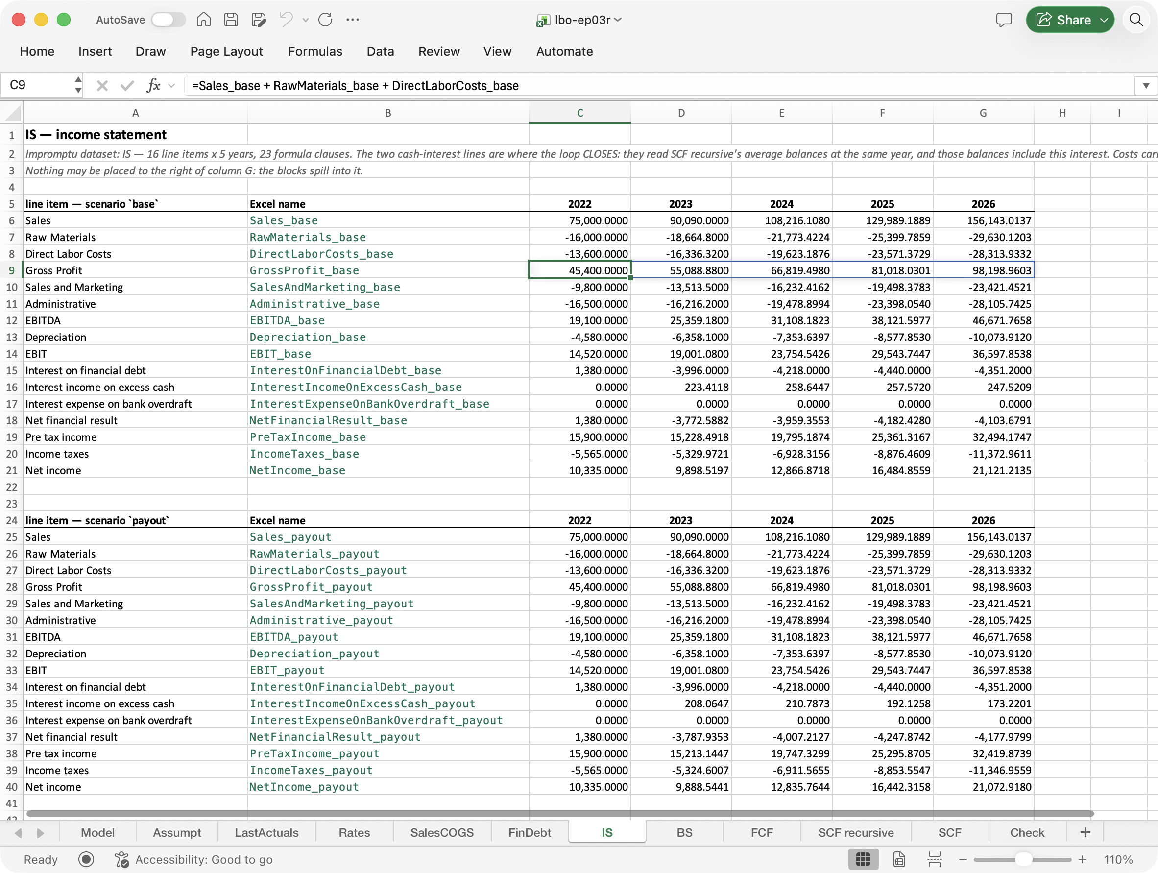
Figure 1: The IS sheet, scenario base. Gross Profit is selected. The formula bar shows its one formula, in C9, and the blue border marks the five years it fills. Column B holds the name each row is given. From row 24 the same block starts again for the scenario payout.

Two constraints come with the layout. A spilled formula needs the cells it spills into to be empty, so nothing may be written to the right of column G, and row 3 of each sheet says so. And the sheet shows values, not the model’s formulas as a list. To give the reader that list, each calculation sheet ends with a translation table: every Impromptu clause, beside the Excel name that reproduces it. On IS it starts at row 63 and counts 23 clauses for 16 formulas, one per line item, written once per scenario (section 4 shows why the counts differ).

3. Inputs go into Tables, calculations cannot

The earlier note recommends Excel Tables for inputs (Layer 0). A Table is a range that Excel knows by name, with named columns, and a formula can refer to a column by its name: tblAssumpt[base] rather than $B$5:$B$31. The three input datasets are Tables here, and so are the model settings. tblAssumpt has one row per assumption and one column per scenario, base, payout and deleverage (Figure 2).

A calculation reads an input through a small function that looks up the label in the Table’s item column and returns the value in the scenario’s column:

IN.ASMPT_base  =LAMBDA(key, FN.PICK(key, tblAssumpt[item], tblAssumpt[base]))
FN.PICK        =LAMBDA(key, keys, vals, XLOOKUP(key, keys, vals, NA(), 0))

so that IN.ASMPT_base("market size g") returns 0.05. The label in quotes plays the part of the coordinate: in Impromptu the same value is Assumpt.market size g. Where a Table has a column per scenario there is one such function per scenario, IN.ASMPT_base, IN.ASMPT_payout and IN.ASMPT_deleverage, because the scenario selects the column. LastActuals has no scenario axis and one function, IN.ACTUAL.

Calculations cannot live in a Table. A line item fills five years across columns, and a Table cannot hold a spilled formula, so the statements are ordinary cells with names, as in section 2.

A second limit splits some input datasets in two. In Impromptu, Assumpt holds 27 inputs and 4 values computed from them, on the same axis: avg sales price = Sales t0 / company sales 000units is a coordinate like any other. In Excel a formula placed in the Table’s base column that calls IN.ASMPT_base reads the whole base column, and so reads itself, which Excel treats as a circular reference, even though the cells it needs are other rows. The four computed values therefore sit below the Table, in rows 35 to 38, each cell with its own name, scoped to the sheet (AvgSalesPrice_base for the scenario base). A calculation reads an input in one of two ways depending on how it is stored: IN.ASMPT_base("Sales t0") for a typed value, Assumpt!AvgSalesPrice_base for a computed one, as another sheet writes it. In Impromptu both are Assumpt.<name>. LastActuals is split the same way, 10 inputs and 4 computed values.

A careful reader may ask why a workbook that names every line item still reads its inputs through labels in quotes. A name for each input and each scenario, written by the build script like the others, would take the labels out of the formulas, at the cost of about ninety more names. Excel’s own tool for naming a whole Table at once, Formulas ▸ Create from Selection, names every row after its label and every column after its header, and market_size_g base then reads one cell. But the names it creates are scoped to the whole workbook, so the base column of Assumpt and the base column of Rates cannot both have one, and the second is silently not created. I kept the labels. In a grid without dimensions, a label in quotes is as close as a formula gets to naming a coordinate.

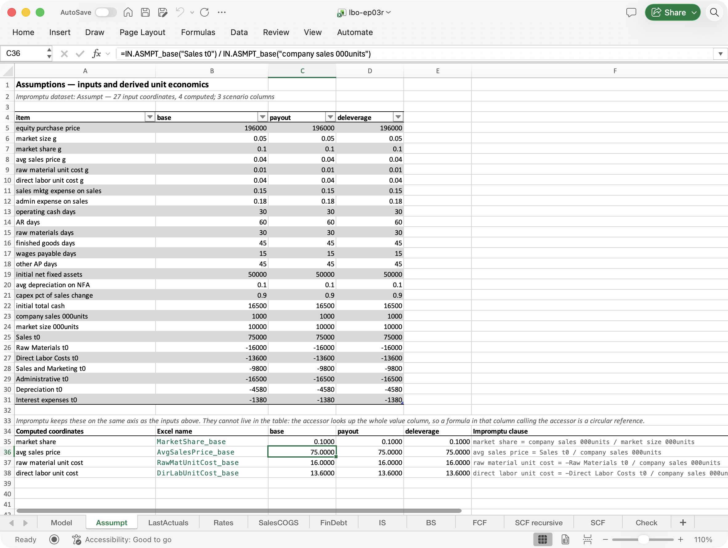
Figure 2: The Assumpt sheet. Rows 4 to 31 are the Table tblAssumpt, one column per scenario. Below it, the four values Impromptu computes on the same axis, which cannot be in the Table. C36 is selected: the formula bar shows avg sales price computed from two inputs read through IN.ASMPT_base.

4. The easy case: one scenario, two axes

The base block of each sheet is what the workbook would be if the model had no scenario dimension: line items by years, which is the shape a grid holds without strain. The names still end in _base. The suffix prepares the workbook for more than one scenario, as the single coordinate base of scenario does in Impromptu. Four examples show how an Impromptu formula becomes an Excel formula, in increasing distance from plain Excel.

A line computed from other lines

Impromptu:

Gross Profit = Sales + Raw Materials + Direct Labor Costs

Excel, in IS!C9 (Figure 1):

=Sales_base + RawMaterials_base + DirectLaborCosts_base

The two say the same thing. Each name refers to a whole row of five years, so the addition is done year by year, and one formula covers the line in both tools. The subtotals of the income statement are all of this kind. The Impromptu formula names no scenario. The Excel formula names base in every operand, and the other two scenarios need formulas of their own (section 5).

A first year that differs from the rest

The first year of the forecast, 2022, is the last actual year, so Sales in 2022 is an input and from 2023 it is computed. Impromptu writes two clauses for the one line item, each naming the years it covers:

Sales[year:first] = LastActuals.Sales
Sales[year:rest] = SalesCOGS.company sales 000units * SalesCOGS.avg sales price

Excel allows one formula per spilled row, so the two clauses have to be joined into one expression (Figure 3):

=FN.SEEDROW(IN.ACTUAL("Sales"), SalesCOGS!CompanySales_base * SalesCOGS!AvgSalesPrice_base)

FN.SEEDROW is one of the workbook’s own functions. It takes the first year’s value and a row computed for all five years, drops that row’s first year and puts the seed in its place:

FN.SEEDROW  =LAMBDA(seed, rest,
               IF(COLUMNS(rest) < 2,
                  seed,
                  HSTACK(seed, DROP(rest, 0, 1))))

The product of quantity and price is computed for 2022 as well, and thrown away.

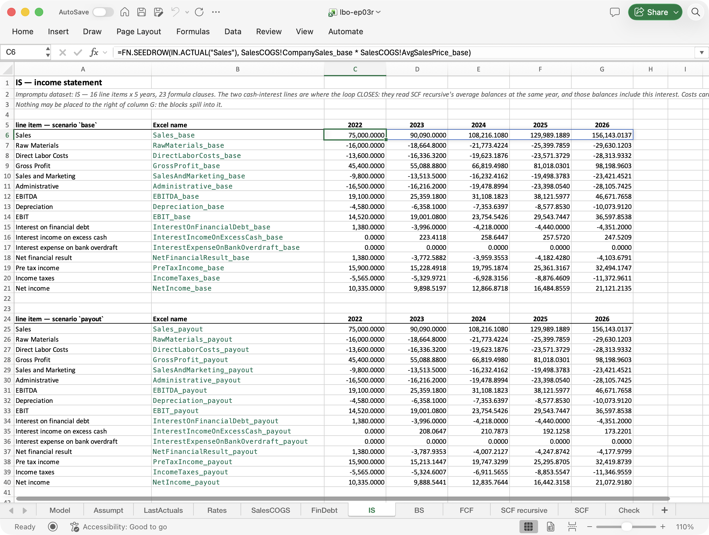
Figure 3: Sales, scenario base. C6 is selected; the formula bar shows the two Impromptu clauses joined by FN.SEEDROW: the 2022 value read from LastActuals, then quantity times price for the years after.

A line that reads its own previous year

Market size grows at a constant rate. Impromptu refers to the previous year of the same line item with [year:prev]:

market size 000units[year:first] = LastActuals.market size 000units
market size 000units[year:rest] = market size 000units[year:prev] * (1 + Assumpt.market size g)

A spilled row that simply referred to its own earlier cells would be a circular reference. In Excel the recurrence is carried by a function that walks the years one at a time: SCAN, as here, or a named LAMBDA that calls itself, which the earlier note also describes (Figure 4):

=FN.GROW(IN.ACTUAL("market size 000units"), IN.ASMPT_base("market size g"), Model!Periods)

FN.GROW takes the seed, the growth rate and the number of years. It turns the single rate into a row of five equal rates with FN.SPREAD, and passes seed and rates to FN.SEEDREC, which keeps the seed as the first year and runs SCAN over the rest, multiplying the previous value by one plus the rate each year. SCAN is the loop the earlier note describes in section 2. Impromptu states the recurrence for one year; the Excel formula names a function that performs it.

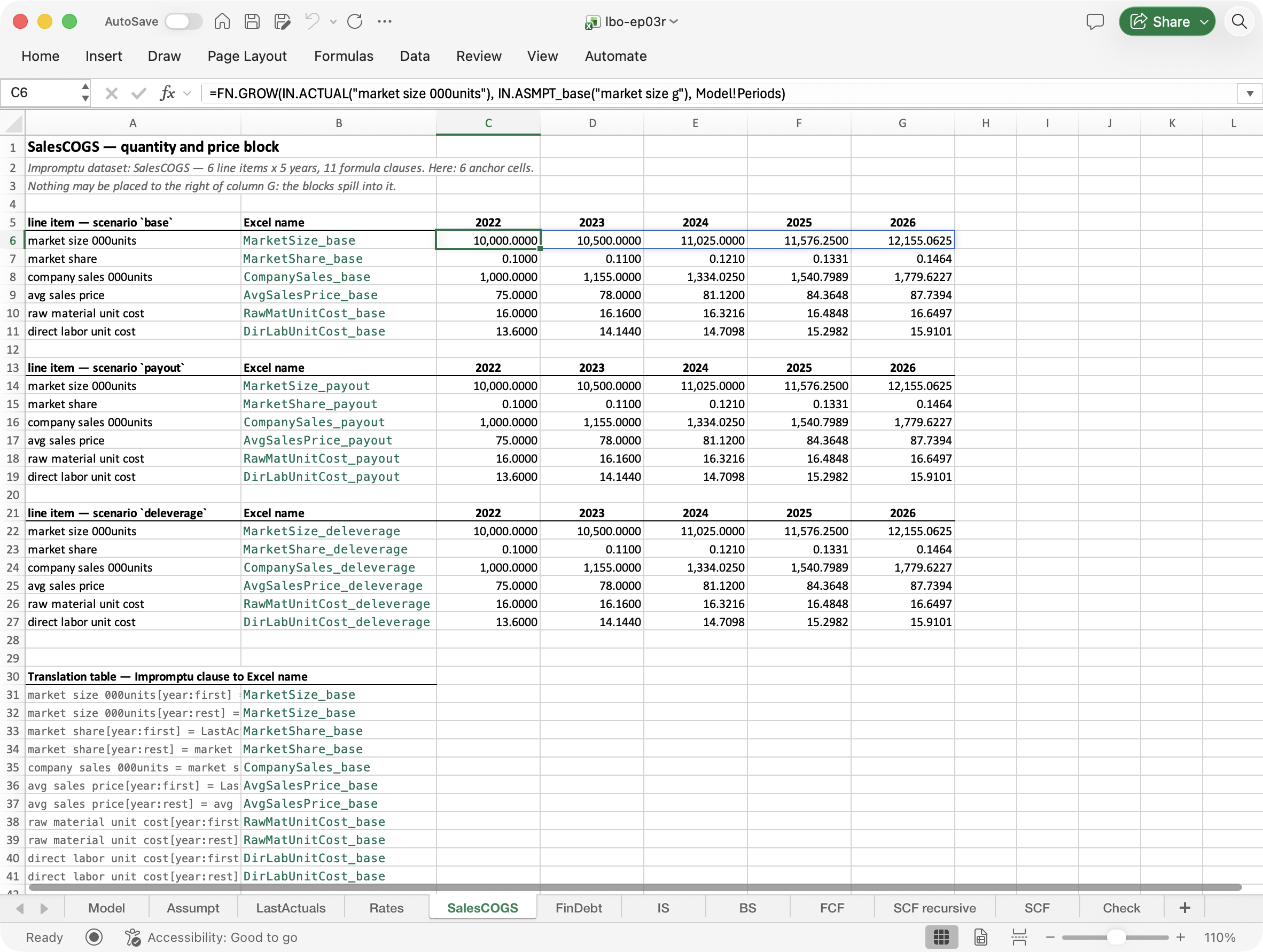
Figure 4: market size 000units on SalesCOGS. C6 holds the whole growth chain in one call to FN.GROW. The three scenario blocks on this sheet are identical: in this model, no scenario changes the market assumptions.

A line computed backwards from the last year

Valuation runs the other way. The unlevered value of the firm in a year is next year’s free cash flow plus next year’s value, discounted at the unlevered cost of capital, and the last year’s value is the continuation value. The valuation is not part of this post’s workbook, but it needs this one more shape, so the example comes from a workbook I built the same way for the valuation of Episode 2. That workbook is not among the downloads. It was built before this one scoped its names to sheets, and its names carry the dataset as a prefix instead: RW. for rWacc V_U, and T.N for the number of years. Impromptu, dataset rWacc V_U:

V_U[year:last] = Continuation Value
V_U[year:butlast] = ( FCFF[year:next] + V_U[year:next]) / ( 1+ rU)

Excel (Figure 5):

=FN.BACKDISC(INDEX(RW.ContinuationValue_base, 1, T.N), RW.FCFF_base, RW.RU_base)

FN.BACKDISC starts from the continuation value in the last year and uses REDUCE to walk from the next-to-last year back to the first, discounting one year at each step. The INDEX(…, 1, T.N) picks the continuation value’s last year, which is what [year:last] says in Impromptu.

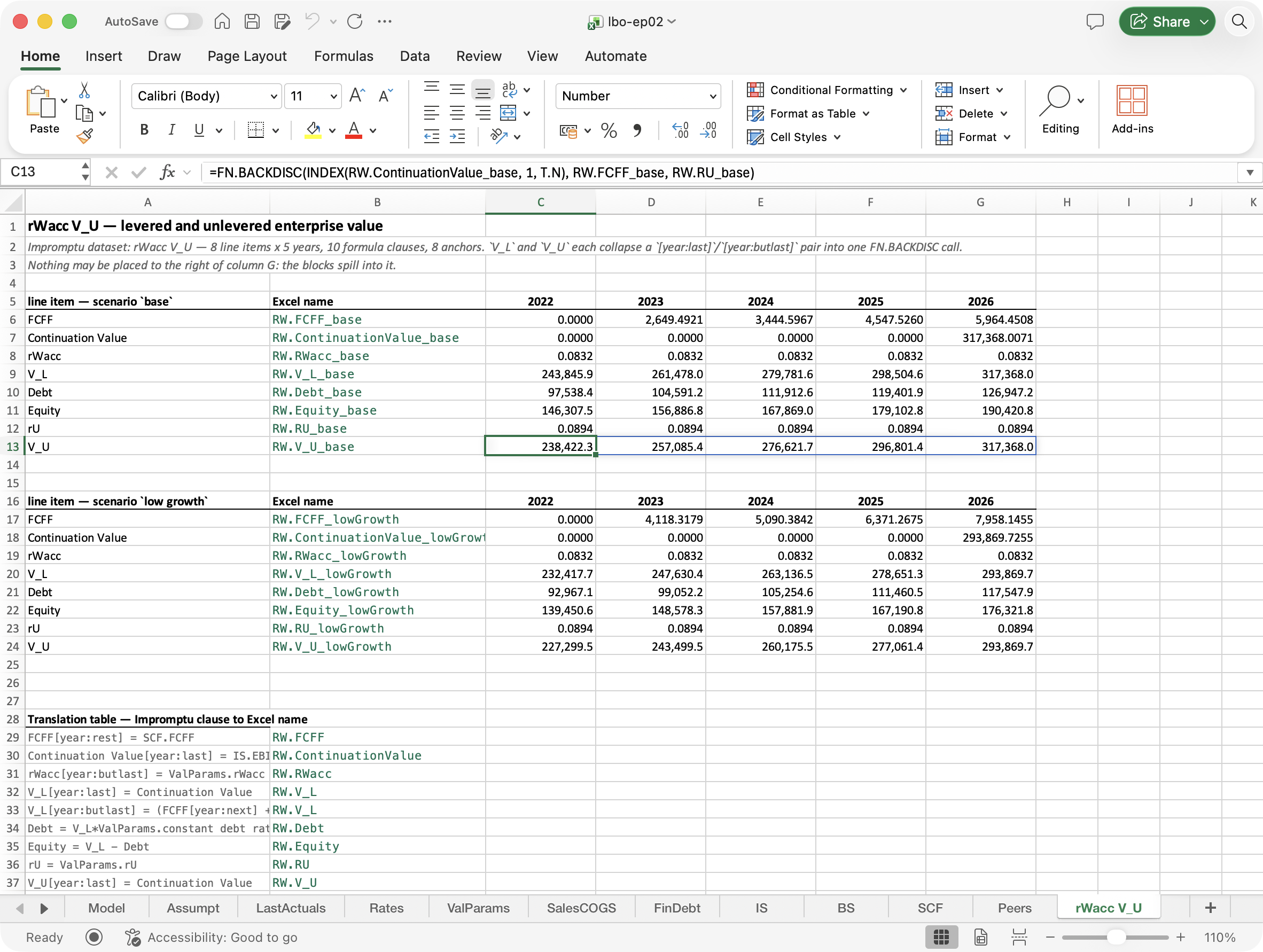
Figure 5: V_U in the valuation workbook. C13 is selected; the formula bar shows the backward recursion as one call to FN.BACKDISC. 2026 holds the continuation value, and each earlier year is discounted from the year after it.

What the wrappers replace

The examples used these functions, one for each form of Impromptu formula that names a position on the year axis:

Impromptu	Excel function	what it does
[year:first] and [year:rest]	FN.SEEDROW	joins a first-year value and the rest into one row
[year:prev] of the same line	FN.SEEDREC, FN.GROW	runs a recurrence forward with SCAN
a single value used for every year	FN.SPREAD	repeats it across the years
[year:last] and [year:next]	FN.BACKDISC	runs a recurrence backward with REDUCE

In Impromptu a clause states the calculation for a year, or a range of years, in the model’s own words. The engine works out the order of the years, the iteration, and how the operands line up. In Excel the modeler chooses a function for each shape of calculation, and the iteration is inside the function. The functions are small and written once, but a reader of the workbook meets one in more than half of the formulas, and has to know what each does to read the model.

5. Adding the scenarios

In Impromptu the three cash policies of Episode 3 are three coordinates of the scenario dimension. When payout and deleverage were added beside base, no formula changed, because every formula applies to every coordinate of the dimensions it spans. No formula of the model names a scenario. The scenarios differ only in their inputs: the share of free cash flow paid as dividends, and the debt repayment schedule.

Excel has no third axis to add a coordinate to, so each scenario gets its own copy of every calculation block. On the IS sheet the base block fills rows 5 to 21, payout starts at row 24 and deleverage at row 43 (Figure 6). Every copy has its own names, with the scenario as the suffix: Sales_base, Sales_payout and Sales_deleverage. The formulas of a copy are those of base with the suffix changed, so Sales under payout reads SalesCOGS!CompanySales_payout * SalesCOGS!AvgSalesPrice_payout. The input Tables have one column per scenario instead, and each scenario has its own lookup functions, as section 3 showed.

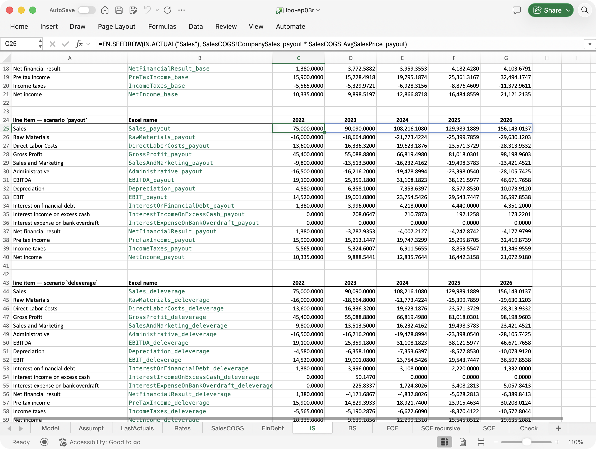
Figure 6: The IS sheet from row 18. The end of the base block, the payout block from row 24 and the start of deleverage at row 43. C25 is selected: Sales under payout is the base formula with every name ending in _payout.

Each scenario after the first adds the same number of names and the same blocks, so the third cost exactly what the second did. Section 12 counts them.

The copies were not typed by hand. The workbook is written by a script from a text description of the model: every formula once, and the list of scenarios on one line. Adding a scenario to that list, with its inputs, writes the new copies with the right names. The description is kept outside the workbook, and the workbook records none of it: nothing in the file says that the three blocks on IS are one object seen under three scenarios.

Who writes the script

Copying the base blocks by hand is a straightforward job: copy a block, paste it below, replace _base with the new suffix in its formulas, and give each row its name. The script does the same, faster and without slips. It was written by an AI assistant, Claude Code, which this series uses throughout: it builds the Impromptu models of the episodes. Here it read the Impromptu model, wrote the description, the script and the checks, and opened the result in Excel to test it, while I reviewed what it did. Almost every step could have been done by hand in Excel; the assistant made them quicker.

The script is written in Python. It writes the .xlsx file with the library xlsxwriter, which stores the formulas, the defined names with their scope, and the Tables, and the checks read the file back with a second library, openpyxl. Excel itself is driven only to recalculate the workbook and read the results. Creating a name and writing a formula over it by hand in Excel is shown step by step in the earlier note; this post starts from a workbook that is already built. Either way, a dimensional model kept in Excel needs work at every change of its structure: a new scenario, line item or dataset means new copies and new names, made by hand, by a script, or by an AI assistant that writes and runs the script.

Excel’s own tools for names are limited. The Name Manager has no search and edits a definition in a one-line box. The add-in that improves it, Excel Labs, is a preview from Microsoft Garage, and I may not install add-ins on my university’s machine. The extension for editing names and LAMBDA functions in VS Code that users have asked for does not exist; the earlier note describes both. A script that writes the names needs neither.

Assistants now also work inside Excel, on the open workbook: Microsoft 365 Copilot, and Anthropic’s Claude for Microsoft 365. An assistant that works outside the spreadsheet, as here, can also write, keep and run the script that generates the workbook. I did not use an assistant inside Excel for this workbook. The last section returns to what these assistants change.

6. Which frictions come from Excel

Sections 3 to 5 met three frictions: constants that have to be turned into rows, formulas wrapped in functions such as FN.SEEDROW, and a copy of the whole model for each scenario. Some of this comes from the way this workbook was built, and some from Excel. They can be taken one at a time.

Constants

Excel already applies a single value to every year of a row. The formula for sales and marketing expense on the income statement is

=FN.SEEDROW(IN.ACTUAL("Sales and Marketing"), -Sales_base * IN.ASMPT_base("sales mktg expense on sales"))

and the rate, one value, multiplies all five years of Sales_base with no wrapper. FN.SPREAD is needed in two places only: where a line item is itself a constant and must still fill five years, and where a function needs a whole row to start from or to walk, as SCAN does and as the fixed point of Part II does. For most formulas the conversion is automatic already.

The first year and the rest

FN.SEEDROW exists because this workbook keeps one formula for each Impromptu line item, so that every line item has its own name, its own row and its own line on the Check sheet. A workbook built directly in Excel could put the first year in a cell of its own and let the formula for the other years spill beside it. The line item would then be two formulas and need a third name to join them. That layout was not built here.

The scenarios

There are five ways to hold a third axis in Excel, and each pays for it in something.

• A copy of every block for each scenario, which is this workbook. Nothing is hidden, and every line item keeps its name. The cost is the copies: without the script of section 5, a new scenario is a copy-and-paste of the whole model, and nothing keeps the copies the same.
• The scenarios as rows inside each block. Each line item becomes a block of three rows, one per scenario, by five years, and Excel’s arithmetic works on the whole block at once. Gross Profit would be one formula for all three scenarios, as in Impromptu, and a new scenario would be a new column in the input Tables and a new row in every block. This is the only layout that reproduces Impromptu’s broadcast inside Excel. It has two costs. Reading one scenario means picking a row by its position, with CHOOSEROWS, and nothing checks that the position is right: a wrong index reads another scenario, with plausible numbers. And SCAN carries one value through a whole block, row after row: run over a block of two rows, it starts the second row from the first row’s last value (measured). A recurrence such as market size would need its own construction to restart for each scenario. This layout was not built (Figure 7).
• One set of sheets for each scenario. The same copies, spread over sheets instead of blocks. Nothing keeps the sheets parallel.
• A switch. One set of blocks, and one input cell that says which scenario the lookup functions read. This is what many working models do, and it is the cheapest. It computes one scenario at a time: two scenarios cannot be seen side by side, no formula can compare them, and the Check sheet could test only the scenario selected. A scenario used this way is a parameter, with one coordinate visible at a time.
• Long format. One table with a column for the scenario, one for the line item, one for the year and one for the value, summarised with GROUPBY or PIVOTBY, as the earlier note describes in Layer 6. Those functions summarise a column that already exists. They cannot compute it, and the values of this model are computed from each other. Long format can be a view of the results; it cannot hold the model.

Figure 7: The scenarios as rows inside each block, a layout this workbook does not use. Each line item is one spilled block of three scenarios by five years, and one formula computes Gross Profit for all three, as in Impromptu. Reading one scenario means picking a row by its position.

There are good reasons to keep a single copy of the calculations, as the switch does. In a multidimensional tool a dimension costs nothing to add while modeling, but it may make the model much larger. A scenario dimension added to a model that was built without one has to be added to every dataset that needs it. Reports across scenarios are often limited, reasonably, to a few key results, and spreadsheets have had what-if tools for that for decades: a data table runs the one calculation once for each set of inputs and tabulates the chosen results. Multidimensional tools do not offer an equivalent natively.

What follows

The frictions of the scenarios come from Excel. The grid has two axes, and every layout above pays for the third in copies, in positions that nothing checks, or in scenarios that cannot be seen together. The wrapper functions are partly this workbook’s own: they are the price of reproducing Impromptu line item by line item, and a model designed in Excel from the start would have fewer of them. Excel’s Beta channel has begun to preview arrays that hold arrays, which may change what the second layout costs. That was not measured here.

The rest of the post takes the first layout as given and asks what happens when the model is circular.

Part II. The circular cash policy

7. The loop

Interest depends on the cash balance. The balance depends on the cash flow of the year. The cash flow depends on the interest. When interest is charged on the year’s average balance, this year’s interest reads this year’s closing balance, and that balance includes this year’s interest. No order of calculation computes every line after the lines it reads.

Modelers usually remove the loop by hand, with a convention that credits interest once a year. Episode 3’s model has both versions, on purpose. The cash flow statement SCF credits interest at year end and has no loop. Its twin SCF recursive accrues interest within the year and has the loop. Episode 3 explains the two conventions and what each costs; Impromptu iterates the model until the values stop changing. The workbook reproduces both statements, each on its own sheet. SCF is built with functions of the kind section 4 showed, plus two for the average balances. SCF recursive is the subject of the rest of this post. This section follows its cash policy line by line, in the scenario base, as the obvious reproduction writes it: one spilled formula per line item, each worded as in Impromptu.

The cash flow before interest

The year starts from the free cash flow to equity, FCFE, computed on the FCF sheet. The company pays a share of it as dividends when it is positive. That share is the dividend policy, one of the two inputs in which the scenarios differ.

Dividends = ifelse(FCFE>=0, -FCFE * Rates.dividends pct of FCFE, 0)
NCF BCI = FCFE + Sale or Purchase of Stock + Dividends + Re-add change in operating cash

=IF(FCFE_base >= 0, -FCFE_base * IN.RATE_base("dividends pct of FCFE"), 0)
=FCFE_base + SaleOrPurchaseOfStock_base + Dividends_base + ReAddChangeInOperatingCash_base

Impromptu’s ifelse becomes Excel’s IF, which also works year by year across the row. NCF BCI is the net cash flow before cash interest, which is what BCI means. None of these lines is in the loop.

The closing balance

The net cash flow adds the interest to the flow before interest, and the cash position accumulates it from the initial cash:

NCF = NCF BCI + After tax cash interest
Net cash position[year:first] = Assumpt.initial total cash
Net cash position[year:rest] = Net cash position[year:prev] + NCF
Discretionary cash = Net cash position - BS.Minimum operating cash
Excess cash = ifelse(Discretionary cash > 0, Discretionary cash, 0)
Bank overdraft = ifelse(Discretionary cash < 0, -Discretionary cash, 0)

The cash position is a recurrence, so Excel writes it with FN.SEEDREC from section 4, this time with the step written in place as a small LAMBDA: the previous balance plus this year’s flow.

=FN.SEEDREC(IN.ASMPT_base("initial total cash"), NCF_base, LAMBDA(prev, d, prev + d))

The cash beyond what the business needs to operate is discretionary. When it is positive it is excess cash, which earns interest; when it is negative it is a bank overdraft, which costs interest. The two ifelse lines become two IF formulas of the same shape as the dividends.

The average balances

Interest is charged on the average balance over the year. The model assumes that the balance moves in a straight line from last year’s close to this year’s. If it stays on one side of zero, the average is the midpoint. If it crosses zero, part of the year is spent in excess cash and part in overdraft, and each part’s average is the area of a triangle divided by the year. Impromptu writes both cases in one formula for each part:

Swing[year:rest] = Excess prev + Excess cash + Overdraft prev + Bank overdraft
Avg excess cash[year:rest] = ifelse(Swing > 0, 0.5 * (Excess prev + Excess cash) * (Excess prev + Excess cash) / Swing, 0)
Avg overdraft[year:rest] = ifelse(Swing > 0, 0.5 * (Overdraft prev + Bank overdraft) * (Overdraft prev + Bank overdraft) / Swing, 0)

The two averages have the same shape, so the workbook writes it once, as the function FN.AVGPART, and calls it twice:

=FN.SEEDROW(0, FN.AVGPART(ExcessPrev_base, ExcessCash_base, Swing_base))

The prev lines are last year’s values, shifted one year to the right by another small function, FN.PREV.

The interest, and back

The interest itself is computed on the income statement, which is where interest belongs:

Interest income on excess cash[year:rest] = Rates.excess cash interest rate * SCF recursive.Avg excess cash
Interest expense on bank overdraft[year:rest] = -(Rates.overdraft interest rate * SCF recursive.Avg overdraft)

=FN.SEEDROW(0, IN.RATE_base("excess cash interest rate") * 'SCF recursive'!AvgExcessCash_base)

SCF recursive reads the two interest lines back from IS, nets them, and takes off the tax:

Cash interest income[year:rest] = IS.Interest income on excess cash
Net cash interest[year:rest] = Cash interest income - Overdraft interest expense
After tax cash interest[year:rest] = Net cash interest * (1 - Rates.tax rate)

=FN.SEEDROW(0, NetCashInterest_base * (1 - IN.RATE_base("tax rate")))

After tax cash interest enters NCF in the second step, in the same year, and the loop is closed: the closing balance gives the average balances, the averages give the interest, and the interest changes the closing balance.

In each forecast year from 2023 to 2026 the loop passes through fourteen line items, two on IS and twelve on SCF recursive (Figure 8). In 2022 there is none, because that year’s interest is an input.

Figure 8: The loop in one year. The fourteen line items that read each other within the same year. The two shaded boxes are on the IS sheet, the other twelve on SCF recursive. Net cash position also reads the previous year’s value, which is outside the loop.

8. The obvious build

The formulas of section 7, one per line item, are the obvious reproduction, and the downloads include it as lbo-ep03r-circ.xlsx. On its SCF recursive sheet the loop is a circle of rows. Row 11, After tax cash interest, reads row 25, Net cash interest, which reads rows 23 and 24, which read rows 16 and 17 of IS, which read the averages in rows 21 and 22, which read the excess cash and overdraft in rows 15 and 16, directly and through the swing in row 20, which read row 14, Discretionary cash, which reads row 13, Net cash position, which reads row 12, NCF, which reads row 11. Each row is one spilled formula for five years, so to Excel every row in the circle reads itself, including the years that are not in the loop.

I expected a spilled range to be unable to take part in a circular reference at all. Excel 16.114 for Mac (Beta channel) does something else. On opening, it shows the dialog of Figure 9 once. The dialog says there is a circular reference and that it cannot list the cells that cause it.

Figure 9: Opening the obvious reproduction. The dialog cannot say which cells form the loop.

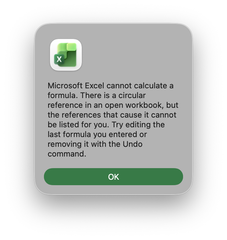
After OK, every line item in the loop reads 0, in every scenario, and so does every line that depends on them. That includes the net cash position of 2022, which is not computed at all: it is the initial cash of 16,500, read from the assumptions. It sits in the same spilled row as the years that are in the loop, and the whole row reads 0 (Figure 10). No cell shows an error value. The status bar says Circular References; when the workbook was first opened by hand and the dialog dismissed, it named a single cell, C91, for a loop that runs across two sheets and three scenarios.

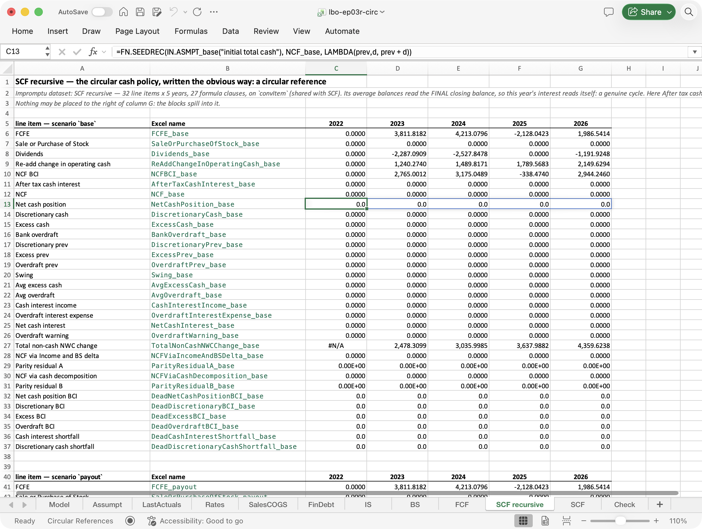
Figure 10: The obvious build, sheet SCF recursive, scenario base. C13 is selected: Net cash position starts from the initial cash of 16,500 and reads 0 in every year, like every other line of the loop. The status bar at the bottom says Circular References.

The zeros look like numbers. A reader who dismissed the dialog sees a model whose cash, interest and overdraft are all zero, and nothing on the sheet says why.

9. Iterative calculation

The classical Excel answer to a circular reference is a setting. On the Mac it is under Excel ▸ Preferences ▸ Calculation, as Use iterative calculation, with a maximum number of iterations and a maximum change. It lets a circular reference stand: Excel recalculates the circle again and again, up to a maximum number of iterations, and stops early when no cell changes by more than a maximum amount. The defaults are 100 iterations and a change of 0.001. Respected modeling standards advise against it. The FAST Standard says never to release a model with purposeful use of circularity, and the ICAEW’s Financial Modelling Code says to disable iterative calculation and resolve circularities with logic. It hides the loop, and it reports nothing about how the calculation ended.

Switched on, it works on the obvious build. The zeros of section 8 are replaced by a cash balance that starts from the initial 16,500 and reaches 25,687.5 in 2026, with interest on the excess cash (Figure 11). A spilled row can take part in iterative calculation like any cell.

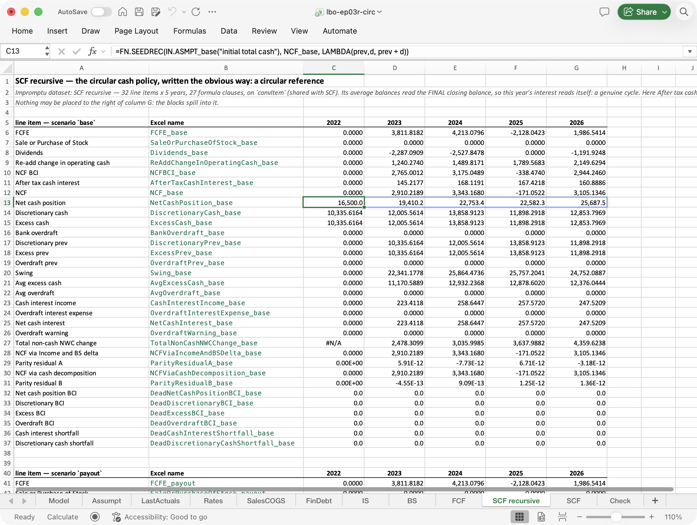
Figure 11: The obvious build with iterative calculation on, at Excel’s default settings. The sheet and the formula are those of Figure 10; Net cash position now starts at 16,500 and every line of the loop has a value.

The values are close to Impromptu’s, but not equal to them at the precision the workbook requires. However many iterations it is allowed, iterative calculation stops improving between 3.8e-9 and 4.5e-9 away from Impromptu’s values, depending on the scenario, so it cannot pass the workbook’s own acceptance limit of 1e-9. At the default settings the scenario deleverage stops 1.7e-6 away. On amounts in thousands both differences are a fraction of a cent. What matters more is that Excel reports neither the difference nor whether the circle settled.

The setting also belongs to Excel rather than to the workbook. The file was saved with iterative calculation on; opened in an Excel that was already running with it off, it read off. One setting governs every open workbook, and the method that solves this model is not part of the model. The next section writes it into the workbook.

10. The fixed point, written in the formula language

With iterative calculation set aside, two ways remain. The model can change, so that the loop disappears: that is what SCF does, by crediting interest once a year, and it changes the economics. Or the workbook can solve the loop itself, in its own formulas. This section does the second.

The idea

Guess the after-tax cash interest for each year. From the guess, compute everything else in the loop: the cash position, the excess cash and the overdraft, the average balances, the interest and the tax. That gives a new after-tax cash interest. If it equals the guess, the guess was right. If not, use the new values as the next guess, and repeat until the change is small enough (Figure 12). A row that the calculation returns unchanged is a fixed point of the loop.

One row is enough because every lap of the loop passes through After tax cash interest (Figure 8), and it has one value per year. It is also the line where the modeler’s own SCF cuts the same loop: SCF computes everything before cash interest and adds the interest once at the end.

Figure 12: The fixed point. A guess for the after-tax cash interest goes through the whole loop and comes back as a new row. The workbook repeats this until the change is below a tolerance, or a cap on the number of iterations is reached.

The loop as a function

In the workbook the guess is a row called atci, and the loop is a LAMBDA of that row. Inside it, LET recomputes the lines of section 7 in the same order and with the same functions, as named intermediate results rather than rows of the sheet:

LAMBDA(atci,
    LET(ncp,     FN.SEEDREC(IN.ASMPT_base("initial total cash"),
                            NCFBCI_base + atci, LAMBDA(prev, d, prev + d)),
        disc,    ncp - BS!MinimumOperatingCash_base,
        exc,     IF(disc > 0, disc, 0),
        od,      IF(disc < 0, -disc, 0),
        exc_p,   FN.SEEDROW(0, FN.PREV(exc)),
        od_p,    FN.SEEDROW(0, FN.PREV(od)),
        swing,   exc_p + exc + od_p + od,
        cii,     IN.RATE_base("excess cash interest rate")
                     * FN.AVGPART(exc_p, exc, swing),
        odie,    IN.RATE_base("overdraft interest rate")
                     * FN.AVGPART(od_p, od, swing),
        FN.SEEDROW(0, (cii - odie) * (1 - IN.RATE_base("tax rate")))))

Line by line: the cash position is the flow before interest plus the guessed interest, accumulated from the initial cash; the discretionary cash is split into excess and overdraft; last year’s values and the swing give the two average balances; the rates give the interest income and the overdraft expense; the tax gives the new row. Everything the function reads from outside, NCF BCI, the minimum operating cash and the rates, lies outside the loop.

The iteration

A second function, written once for any loop, applies the first one repeatedly:

FN.FIXPOINT  =LAMBDA(step, seed, tol, cap,
               REDUCE(HSTACK(seed, 0, 1E+300), SEQUENCE(cap),
                 LAMBDA(acc, k,
                   LET(n,    COLUMNS(acc) - 2,
                       x,    TAKE(acc, 1, n),
                       last, INDEX(acc, 1, n + 2),
                       IF(last <= tol,
                          acc,
                          LET(y,     step(x),
                              big,   IF(ABS(x) > ABS(y), ABS(x), ABS(y)),
                              denom, IF(big > 1, big, 1),
                              HSTACK(y, k, MAX(ABS(y - x) / denom))))))))

REDUCE walks through the numbers 1 to cap carrying an accumulator: here, the current row followed by two cells, the number of iterations used and the last change. At each step TAKE(acc, 1, n) takes the row out of the accumulator as x, and step(x) passes it to the loop function of the previous listing, where it is the argument atci. What comes back, y, is the new after-tax cash interest. The change is measured the way Impromptu measures it: the largest difference between x and y, relative to the larger of 1 and the two values. REDUCE cannot stop early, so once the change is below the tolerance each remaining step returns the accumulator as it is, without running the loop again. The first guess, seed, is a row of zeros.

Excel already has functions that work this way. IRR looks for the rate at which the net present value of a series of cash flows is zero. No formula gives that rate directly, so IRR starts from a guess and iterates inside the function: Microsoft documents that it cycles until the result is accurate within 0.00001 percent, and returns #NUM! if it has not found one after 20 tries. The sheet sees one ordinary formula; the iteration is hidden inside it. FN.FIXPOINT does the same for the cash policy. It looks for the row for which step(x) equals x, which is the same as looking for a zero of step(x) - x, and it iterates inside a function that reads only values outside the loop. The loop leaves the workbook’s recalculation, where Excel could only report a circular reference, and runs inside one formula, where the modeler sets the tolerance and the cap and can see how many iterations it took.

The tolerance, 1e-14, and the cap, 50 iterations, are inputs on the Model sheet. The tolerance is a modeling decision. It is tighter than Impromptu’s own setting, because at Impromptu’s tolerance the scenario deleverage stops earlier and lands just outside the workbook’s acceptance limit.

On the sheet

Row 11 of SCF recursive holds the call, FN.FIXPOINT(step, zeros, Model!FixTol, Model!FixCap) with the function above as step. It spills seven cells: the five years of the row, then the iterations used and the last change (Figure 13). Row 12, After tax cash interest, takes the five years from it:

=TAKE(FixedPoint_base, 1, Model!Periods)

Every other row is the formula of section 7, unchanged. The circle is gone, because row 12 now reads the solver, and the solver reads nothing inside the loop. The visible rows compute the loop a second time from the solved row, and they return the same row: section 12 gives the check.

The fixed point takes 9 iterations for base and payout and 12 for deleverage, and the whole workbook agrees with Impromptu within the acceptance limit.

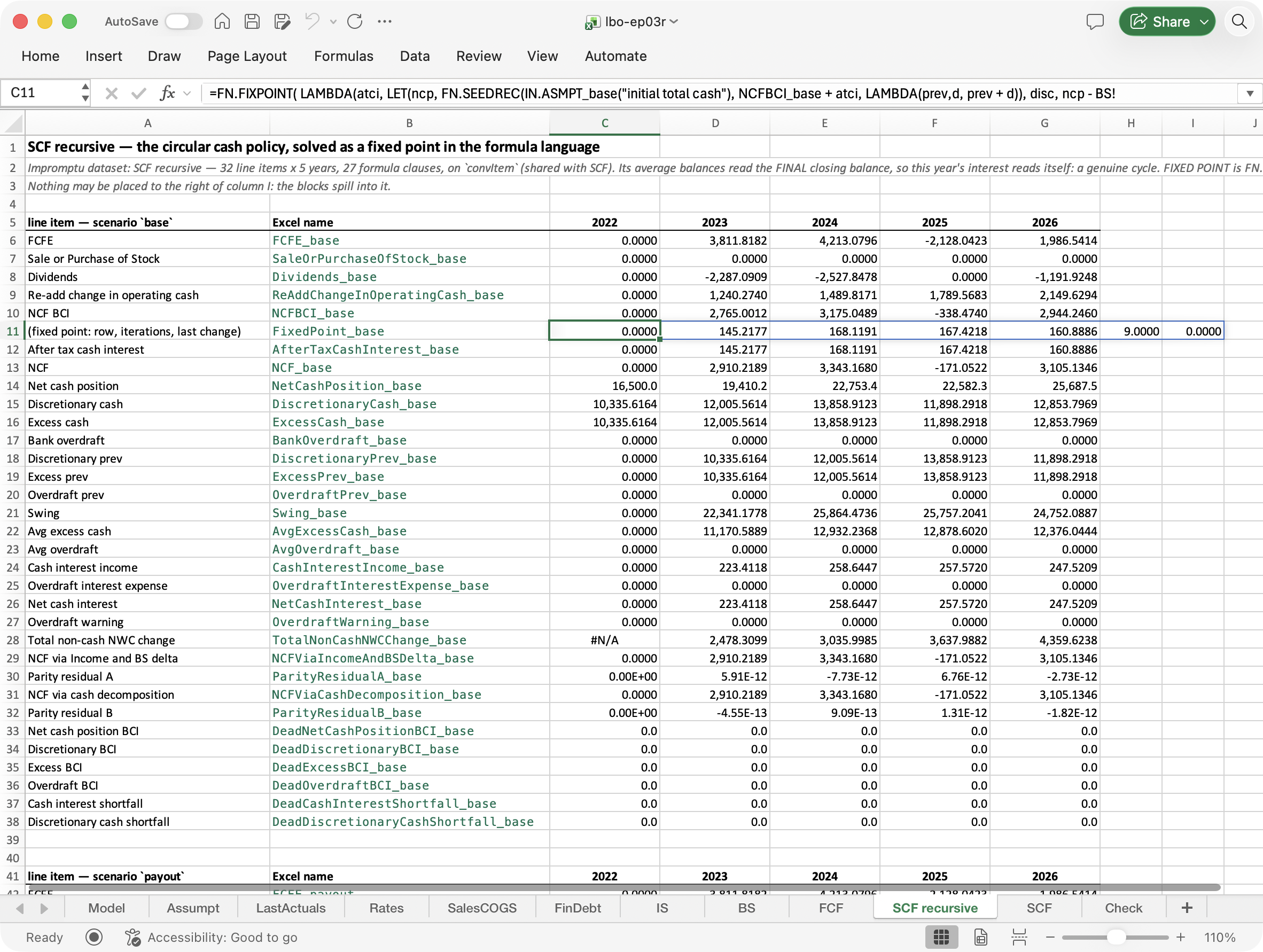
Figure 13: The solved workbook, sheet SCF recursive, scenario base. C11 is selected, and the formula bar shows the start of the call to FN.FIXPOINT. Row 11 is the fixed point: the five values of After tax cash interest in columns C to G, then 9 iterations in column H and a last change that displays as 0 in column I. Row 12 reads its values from row 11, and the rows below are those of Figure 10, now with values.

11. Each scenario converges on its own

The fixed point is part of the base block, and like every block it is copied once per scenario (section 5). SCF recursive has three solver rows, one at the top of each block:

scenario	solver row	iterations (column H)
base	C11:I11	9
payout	C47:I47	9
deleverage	C83:I83	12

Each copy stops when its own scenario has converged. deleverage is the scenario that repays its debt fast enough to run an overdraft: its balance crosses zero in 2023, and from then on it pays 8% on an overdraft instead of earning 2% on excess cash. It is also the one that takes longest, in Excel as in Impromptu.

Impromptu does it the other way. The three scenarios are coordinates of the same arrays, and the engine converges them together, so all three take as many passes as the slowest, 12, as Episode 3 reports. Excel’s iterative calculation of section 9 is one setting for the whole workbook, so it too runs until the slowest scenario has settled.

So the copies that the missing dimension forces on the workbook have one effect in its favour: each scenario pays only for its own convergence. I did not measure what that saves in time.

12. What it cost, in numbers

This section collects the measurements the rest of the post refers to. A reader who does not need them can skip to section 13. Every number is read from the workbook as it ships, from the scripts that build and check it, or from the Impromptu model it reproduces. The measurements were made on Excel 16.114 for Mac (Beta channel), and the acceptance check was run again on 16.115 on the workbooks as they ship.

Acceptance

The workbook covers the ten datasets of the forecast. They hold 140 formula clauses in Impromptu; 139 are rebuilt as Excel formulas and one, the cost of debt, is typed in.

The Check sheet compares 524 line items in 43 blocks: 14 groups of line items for each of the three scenarios, and LastActuals once. Thirty-six cells for which Impromptu has no value are compared as absent. The acceptance limit is an absolute difference of 1e-9, and the largest difference is 5.82e-11. The sheet also checks the model’s own identities: the balance sheet balances to 0 in every year and scenario, and the two cash-flow reconciliations of Episode 3 agree to about 1e-11, which is the size of the rounding in sums of this magnitude, in Excel as in Impromptu. With the workbook switched to Excel’s Compatibility Version 3, which previews nested arrays, every result is the same.

The formulas

The base blocks hold 135 formulas. 60 use none of the workbook’s own functions, 54 use FN.SEEDROW, and 75 use at least one function. The library the workbook carries has 17 functions in 96 lines of formula. 184 formulas read an input through a label in quotes, 39 labels in all: 23 of Assumpt‘s 27 rows, 9 of LastActuals’ 10, the 5 rates and the 2 settings.

The names of the third axis

The workbook has 539 defined names. Built with one scenario it would have 199, and with two, 369: each scenario after the first adds 170, of which 139 are the line items that vary by scenario. Of the 539, 433, or 80%, exist only because the grid has no dimensions. They are of four kinds, each with what Impromptu has instead:

kind	names	in Impromptu
one name for each distinct line item	143	a coordinate of its dataset
the copies of those names for payout and deleverage	278	a coordinate of scenario
functions that look a label up in a Table	9	the label is the address
the years: start, count and row	3	the dimension year

The other 106 are the library, the Check sheet and the fixed point. A reader who does not accept one of the kinds can subtract it.

Scoping the names to their sheets moves no name from one kind to another. Of the 539, 517 are scoped to a sheet: Model 5, Assumpt 12, LastActuals 4, SalesCOGS 18, FinDebt 6, IS 48, BS 96, FCF 45, SCF recursive 99, SCF 96 and Check 88. The other 22 are the functions, scoped to the workbook. The 143 names of the first kind are now pairs of a sheet and a name, and they use 104 distinct spellings, because the same short name lives on several sheets, as a line item of the same name lives in several Impromptu datasets. Excel still spends a name on each of them.

Iterative calculation, measured

Measured on the obvious build, starting from the zeros, with the maximum change set to 0 so that only the number of iterations stops Excel. The deviation is the largest difference of Discretionary cash from Impromptu over the five years.

iterations	base	payout	deleverage
1 or 2	6.4e+2	5.1e+2	6.7e+3
9 or 10	4.9e-5	4.3e-5	3.8e-2
15 or 16	4.45e-9	3.84e-9	1.7e-6
19 to 100	4.45e-9	3.84e-9	4.47e-9
Excel’s defaults (100, change 0.001)	4.45e-9	3.84e-9	1.7e-6

The deviations come in identical pairs: each step of progress takes two Excel iterations. Below about 4.5e-9 the values stop improving, which is above the acceptance limit.

The fixed point

The fixed point costs 13 lines of library formula for FN.FIXPOINT, 5 for FN.AVGPART, and 14 lines for the step, the loop written as a function. It adds six defined names: the function, the tolerance, the cap, and one solver row per scenario. The solver’s row and the same row recomputed by the visible sheets from it differ by at most 5.7e-14.

The tolerance was chosen, not copied. Swept on the same construction:

tolerance	base	payout	deleverage
1e-10, Impromptu’s	7 iterations, 4.7e-11	7, 4.4e-11	9, 1.9e-9
1e-12	8, 3.6e-12	8, 3.6e-12	10, 5.8e-11
1e-14, shipped	9, 3.6e-12	9, 3.6e-12	12, 4.5e-13

The deviation here is that of the net cash position from Impromptu’s saved values, computed by a Python copy of the same arithmetic. At Impromptu’s own tolerance deleverage lands outside the 1e-9 limit. The same change made in Excel, to Model!FixTol, gives the same iteration counts at every tolerance. At 1e-10 the Check sheet’s worst deviation over all 43 blocks reads 2.11e-9, and its verdict reads FAIL; the video makes this change on camera.

Iterations to converge, from zeros, by scenario:

	base	payout	deleverage	the model pays
Impromptu	10	10	12	12, together
Excel iterative calculation, to its floor	13 to 15	13 to 15	19	19, one setting
FN.FIXPOINT	9	9	12	each its own

The Impromptu counts are those of its default mode, per scenario from one run of the three together (Episode 3 gives the counting rule).

Which row to iterate

The loop has fourteen line items in each year. A fixed point has to guess enough of them to break every lap, and the fewer it guesses the smaller the accumulator REDUCE carries. That question was answered before any formula was written, by a dependency checker that reads the Impromptu model, draws the graph of line items and years, and finds the smallest sets of line items whose removal breaks every cycle. Here one line item is enough, and five different ones would each do: After tax cash interest, Discretionary cash, NCF, Net cash interest and Net cash position. The workbook uses the first, where the modeler’s own SCF cuts the loop.

The machinery outside the workbook

The dependency checker is part of the machinery that builds and checks the workbook: a text description of the model, and the scripts that generate the workbook from it, refuse a plan with a loop nobody declared, and open the result in Excel to compare it with Impromptu. Counted as all lines of the build and check scripts, the machinery is 5,514 lines of Python, against the 96 lines of formula it builds into the workbook: about 57 times as much. The scripts were written by the AI assistant of section 5, and none of them is in the workbook. They are kept in my own repository, which is not public. By path:

• excel-models/lbo-ep03r/spec/model.py: the text description of the model;
• excel-models/_shared/lib/*.lambda: the function library, one file per function;
• excel-models/_shared/build/build.py: the build, which writes the workbook with xlsxwriter;
• xlformula.py: formula text to the form stored in the file, and the checks on it;
• depgraph.py: the dependency graph of line items and years, and the order of the blocks;
• extract_expected.py: the expected values, read from the Impromptu model;
• excel_check.py and excel_stage.py: the acceptance check, run inside Excel on a copy of the workbook;
• census.py and scope_census.py: the counts of names above;
• rescope.py: the move from prefixed names to names scoped to their sheets, and its proof that every formula is the old one renamed;
• source_readback.py: the formulas Excel displays, compared with the description.

All but the first two are in excel-models/_shared/build/. A script must also write some things the way Excel stores them rather than the way a person types them: a name whose definition reads another sheet-scoped name carries that name’s sheet, even when both are on the same sheet.

What the engine does instead

The Impromptu model carries two settings for its loop: a maximum of 100 iterations and a tolerance of 1e-10. The engine finds the loop, orders the rest of the calculation around it, and iterates it. Nobody writes a step function, chooses a row to guess, or sets a cap for each scenario.

13. What it takes

The earlier note ended on a narrow correction. Modern Excel has adopted the formula idea of the multidimensional tools, one rule for a whole line item, and not the data idea, dimensions that the engine knows by name. Of the six properties the note used to compare the two (its scorecard), Excel had the first, one rule per line, and only parts of the rest. And what Excel lacks has to be maintained by the modeler, where a multidimensional engine enforces it (section 10).

This rebuild tested that conclusion on a real model, and it held. The model of Episode 3 can be rebuilt in Excel with formulas only, and the workbook agrees with Impromptu within the limit it sets itself; the two workbooks of the next section let a reader check that. One rule per line item is there: one spilled formula for each line, and Gross Profit reads the same in both tools. The dimension is not quite there. The scenarios are copies, the positions on the year axis are functions the workbook carries, and the coordinates of an input are labels in quotes. The copies, the names and the labels stay consistent because a script writes them, not because Excel knows what they stand for.

Section 6 separated what comes from Excel from what comes from this reproduction. The copies come from Excel; the wrapper functions are partly the price of rebuilding Impromptu line item by line item.

The loop takes decisions Excel does not make. Written the obvious way it computes as zeros. Iterative calculation solves it closely, from a setting that belongs to Excel rather than to the workbook, and says nothing about how it ended. The fixed point of section 10 solves it inside the workbook, in one formula per scenario, like IRR. It is small, and it rests on choices made before it was written: which row to guess, what tolerance to accept, how many iterations to allow.

The settings the modeler should not have to touch

Every tool that solves a loop has settings. Excel has the calculation mode, automatic or manual, iterative calculation on or off, its maximum number of iterations and maximum change, and the number of calculation threads. Impromptu’s model has a maximum number of iterations and a tolerance, and the engine has two recalculation modes. The model of Episode 3 was built without touching any of them: the engine found the loop and iterated it. In the Excel workbook two of those settings, the tolerance and the cap, became inputs on the Model sheet, and choosing them was part of building the model.

The assistant

The scripts that write the copies, the check against Impromptu and the fixed point were written by an AI assistant, with me reviewing. Almost every step could have been done by hand. The assistant made the work quicker; it did not change what the workbook is.

14. The workbooks, to download

The two workbooks of this post can be downloaded and opened. They use LAMBDA and the array functions of recent Excel, so they need Microsoft 365 or Excel 2024. They contain no macros and need no add-in. They were built and checked on Excel 16.115 for Mac (Beta channel), and have not been tested on Windows.

• lbo-ep03r.xlsx is the circular model, solved by the fixed point. The places to look first:
  • the IS sheet, column C: one formula per line item, and the name of each row in column B (section 2);
  • Formulas ▸ Name Manager: every line item, every copy for the other two scenarios, and the workbook’s own functions (sections 2 to 5). The Scope column gives each name’s sheet, and Filter ▸ “Names Scoped to Worksheet” leaves out the functions. The list is in alphabetical order, so the three copies of a line item, such as Sales_base, Sales_deleverage and Sales_payout, sit together. The Name Manager has no search box: typing a letter with the list selected moves to the first name that starts with it. To reach a line item, type its name with its sheet, IS!Sales_base, in the Name Box, the box left of the formula bar that shows the cell’s address, and press Enter. The Name Box does not complete the name, and its drop-down lists only the Tables and the functions;
  • the SCF recursive sheet, row 11: the fixed point for the scenario base, the five values of After tax cash interest, then the iterations used and the last change; the blocks for payout and deleverage start at rows 47 and 83 (sections 10 and 11);
  • the Model sheet, rows 15 and 16: the tolerance and the cap of the fixed point, which can be changed;
  • the Check sheet: cell B4 holds the largest difference from Impromptu, and D4 reads PASS when it is at most 1e-9. A #N/A marks a cell for which Impromptu has no value, mostly in 2022, where a change from the previous year has no previous year. The Name Manager’s Filter ▸ “Names with Errors” lists the 12 expected-value ranges that hold these cells, four per scenario. They hold #N/A on purpose: a value present on only one side then counts as a mismatch instead of being skipped.
  The inputs are in the Tables on Assumpt, LastActuals and Rates. Change one and every sheet recomputes; the Check sheet then no longer applies, because its expected values are Impromptu’s for the inputs as shipped.
• lbo-ep03r-circ.xlsx is the obvious reproduction of section 8. It opens with the dialog of Figure 9 and computes the loop as zeros. Switching on iterative calculation (section 9) gives it values.

---

Glossary

Dynamic arrays, spilled ranges, LET, LAMBDA and the functions that take one are explained, with examples, in section 2 of the earlier note. The entries below are the terms this post adds.

Scenario

A coordinate of the dimension scenario. In Impromptu one formula covers every scenario; in this workbook each scenario has its own copy of every calculation block. The three scenarios of Episode 3 are cash policies: base, payout and deleverage.

Defined name

A name given to a cell, a range or a formula in the Name Manager (Formulas ▸ Name Manager), usable in any formula of the workbook in place of an address. Every line item of this workbook has one, such as GrossProfit_base, referring to its whole spilled row.

Scope

The part of the workbook in which a defined name is known. A name scoped to a sheet is written plainly on that sheet and with the sheet in front elsewhere: GrossProfit_base on IS, IS!GrossProfit_base on any other sheet. It plays the part of an Impromptu dataset, inside which a line item is named without the dataset (section 2). A name scoped to the workbook, such as a function’s, is written the same way everywhere.

Excel Table

A range that Excel knows by name, with named columns, created with Insert ▸ Table. A formula can refer to a column by name (tblAssumpt[base]). A Table cannot hold a spilled formula, so in this workbook it holds inputs only.

Lookup function

In this workbook, a small LAMBDA that finds a label in a Table and returns the value in one scenario’s column, such as IN.ASMPT_base("market size g"). The label plays the part of an Impromptu coordinate.

Circular reference

A formula that reads, directly or through others, its own result. Excel reports one on opening and, unless iterative calculation is on, computes the cells involved as zeros (section 8).

Iterative calculation

An Excel setting that lets a circular reference stand and recalculates it repeatedly, up to a maximum number of iterations or until no cell changes by more than a maximum amount (by default 100 and 0.001). It belongs to Excel rather than to the workbook (section 9).

Fixed point

A value, here a row of values, that a calculation returns unchanged. A circular model is solved by finding one: start from a guess, apply the model to it, and repeat with the result until it stops changing. In this workbook FN.FIXPOINT does it inside one formula (section 10).

Tolerance and cap

The two settings of a fixed-point search: how small the change must be to stop, and the largest number of iterations allowed. In this workbook they are inputs on the Model sheet, 1e-14 and 50.

Build script

The program that writes this workbook from a text description of the model, including one copy of every block per scenario, and checks the result against Impromptu. It is kept outside the workbook (sections 5 and 12).